Writing Reproducible Research Papers with R Markdown
Resul Umit
24 May 2022
Who am I?
Resul Umit
post-doctoral researcher in political science at the University of Oslo
teaching and studying representation, elections, and parliaments
- a recent publication: the effects of casualties in terror attacks on elections
Who am I?
Resul Umit
post-doctoral researcher in political science at the University of Oslo
teaching and studying representation, elections, and parliaments
- a recent publication: the effects of casualties in terror attacks on elections
teaching workshops, also on
Who am I?
Resul Umit
post-doctoral researcher in political science at the University of Oslo
teaching and studying representation, elections, and parliaments
- a recent publication: the effects of casualties in terror attacks on elections
teaching workshops, also on
- more information available at resulumit.com
How did I use to write?
First, with Stata + Word, I was ...
frustrated with Word
- formatting tables, figures, citations, and equations
- managing references
tired of switching between programmes/screens
- and, worried about making mistakes in between
paying for programme licences
How did I use to write?
Then, with Stata + R + LaTeX, I was ...
frustrated with Wordformatting tables, figures, citations, and equationsmanaging references
tired of switching between programmes/screens
- and, worried about making mistakes in between
paying for the Stata licence
converting PDF documents to Word manually
- coordinating work with co-authors who don't use LaTeX/PDF
- submitting to journals which don't accept LaTeX/PDF
How do I write now?
Now, with R Markdown, I am ... happy!
frustrated with Wordformatting tables, figures, citations, and equationsmanaging references
tired of switching between programmes/screensand, worried about making mistakes in between
paying for the Stata licenceconverting PDF documents to Word, manuallycoordinating work with co-authors who don't use LaTeX/PDFsubmitting to journals which don't accept LaTeX/PDF
R Markdown
Efficient
- write text, cite sources, tidy data, analyse, table, and plot it in one programme/screen
- re-do one, more, or all of these with ease
- decrease the possibility of making mistakes in the process
R Markdown
Efficient
- write text, cite sources, tidy data, analyse, table, and plot it in one programme/screen
- re-do one, more, or all of these with ease
- decrease the possibility of making mistakes in the process
Flexible
- output to various formats
- e.g., HTML, LaTeX, PDF, Word
- output to various formats
Open access/source
- use for free
- create documents accessible to anyone with a computer and internet connection
- benefit from the work of a great community of users/developers
Reproducibilty — Before Publication
Having written a complete draft
- with data including re-coded variables, tables, figures, and text with references to specific results (e.g., numbers from summary and/or regression statistics)
Reproducibilty — Before Publication
Having written a complete draft
- with data including re-coded variables, tables, figures, and text with references to specific results (e.g., numbers from summary and/or regression statistics)
If you and/or your co-authors decide
- to reverse a re-coded variable to its previous/original measure
- and/or, to exclude a subgroup of observations from analysis
How resource intensive would this revision be?
- how long would this revision take?
- how many programmes would be needed for this revision, and how much would they cost?
- there is an inverse relationship between this resource intensity and reproducibilty
Reproducibilty — After Publication
After your paper is published, if others, including your future self, would like to test how robust the results are
- to reversing a re-coded variable to its previous/original measure
- and/or, to excluding a subgroup of observations from analysis
Reproducibilty — After Publication
After your paper is published, if others, including your future self, would like to test how robust the results are
- to reversing a re-coded variable to its previous/original measure
- and/or, to excluding a subgroup of observations from analysis
How resource intensive would this test be?
- how accessible is the data, documentation (how was the variable re-coded in the first place?), and the code?
- how long would the test take?
- how many programmes would be needed for this revision, and how much would they cost?
- there is an inverse relationship between this resource intensity and reproducibilty
The Workshop — Overview
Two days, on how to write reproducible research papers with R Markdown
- 200+ slides, 40+ exercises, and time for converting a real project
The Workshop — Overview
Two days, on how to write reproducible research papers with R Markdown
- 200+ slides, 40+ exercises, and time for converting a real project
Based on converting a mock manuscript written in Word to R Markdown
- plus, improving its reproducibility and version-controlling it
- with a PDF output in mind
Designed for researchers with basic knowledge of R programming language
- does not cover programming with R
- e.g., writing functions
- e.g., writing functions
- ability to regress, plot, and table in R will be very helpful
- but not absolutely necessary — these skills can be developed after learning R Markdown as well
- does not cover programming with R
The Workshop — Contents
Part 1. Getting the Tools Ready
- e.g., downloading course material
Part 2. Introducing R Markdown
- e.g., creating a new document
- e.g., defining output format
- e.g., adding emphasis to text
- e.g., citing sources
The Workshop — Contents
Part 1. Getting the Tools Ready
- e.g., downloading course material
Part 2. Introducing R Markdown
- e.g., creating a new document
- e.g., defining output format
- e.g., adding emphasis to text
- e.g., citing sources
Part 6. Adding Code, Figures, and Tables
- e.g., plotting data
Part 7. Addressing Functionality Gaps
- e.g., adjusting line spacing
- e.g., integrating Git and GitHub
Part 9. Collaborating with Others
- e.g., working simultaneously with co-authors
Part 10. Working on a Real Project
- e.g., converting a work-in-progress of yours
The Workshop — Organisation
Sit in groups of two
- participants learn as much from their partner as from instructors
- switch partners after every second part
Type, rather than copy and paste, the code that you will find on these slides
- typing is a part of the learning process
When you have a question
- ask your partner
- google together
- ask me
The Workshop — Organisation — Slides
Slides with this background colour indicate that your action is required, for
setting the workshop up
- e.g., downloading course material
completing the exercises
- e.g., managing references in R Markdown
- there are 40+ exercises
- these slides have countdown timers
03:00
The Workshop — Organisation — Slides
Codes and texts that go in R Markdown documents appear as such — in a different font, on gray background
- long codes and texts will have their own line(s)
```{r, scatterplot, fig.cap = "A scatterplot of journal metrics."}ggplot(data = df, mapping = aes(x = h5_median, y = h5_index, color = subfield)) + geom_point() + facet_wrap(. ~ branch) + scale_colour_discrete(name = "Journal Type", breaks = c(0, 1), labels = c("Generalist", "Subfield")) ```The Workshop — Organisation — Slides
Codes and texts that go in R Markdown documents appear as such — in a different font, on gray background
- long codes and texts will have their own line(s)
Results that come out in output files appear as such — in the same font, on green background
- except very obvious results, such as figures and tables
The Workshop — Organisation — Slides
Codes and texts that go in R Markdown documents appear as such — in a different font, on gray background
- long codes and texts will have their own line(s)
Results that come out in output files appear as such — in the same font, on green background
- except very obvious results, such as figures and tables
Specific sections are highlighted yellow as such for emphasis
- these could be for anything — codes and texts in input, results in output, and/or texts on slides
The slides are designed for self-study as much as for the workshop
- accessible, in substance and form, to go through on your own
The Workshop — Aims
To make you aware what is possible with R Markdown
- we will cover a large breath of issues, not all of it is for long-term memory
- one reason why the slides are designed for self study as well
- one reason why the slides are designed for self study as well
- awareness of what is possible,
Google, and perseverance are all we need
- we will cover a large breath of issues, not all of it is for long-term memory
To encourage you to convert into R Markdown
- practice with a mock manuscript (Parts 3–9)
- start converting a real one (Part 10)
Course Materials — Download from the Internet
Download the materials from https://github.com/resulumit/rmd_workshop/tree/materials
- on the webpage, follow
Code -> Download ZIP
Unzip and rename the folder
unzip to a location that is not synced
- e.g., perhaps Documents, but not Dropbox
rename the folder as
YOURNAME-rmd- e.g.,
resul-rmd - this will come handy when we collaborate Part 9
- e.g.,
Course Materials — Overview
Notice that the folder has the following structure
YOURNAME-rmd | |- manuscript | | | |- reproduce_this.pdf | |- journals.Rmd | |- references.bib | |- apa_7th.csl | |- data | | | |- journals.csv | |- image | | | |- google_scholar.pngCourse Materials — Contents
manuscript\reproduce_this.pdf- the document, formatted in Word but saved as PDF, that we will re-create with R Markdown
- randomly generated sentences, with figures and tables from randomly a generated dataset*
- key sections in need of attention are highlighted yellow
* The text, Lorem ipsum, is generated with the stringi package (Gagolewski, Tartanus, Unicode, Inc., and others, 2021) while the dataset is created with the fabricatr package (Blair, Cooper, Coppock, Humphreys, Rudkin, and Fultz, 2022).
Course Materials — Contents
manuscript\reproduce_this.pdf- the document, formatted in Word but saved as PDF, that we will re-create with R Markdown
- randomly generated sentences, with figures and tables from randomly generated dataset
- key sections in-need of attention are highlighted
manuscript\journals.Rmd- the R Markdown document that we will work on
- includes unformatted text from
reproduce_this.pdfto save time - major components, such as paragraphs and tables, are numbered and marked in comments to facilitate navigation
manuscript\references.bib- a BibTeX document with three fabricated references
manuscript\apa_7th.csl- a Citation Style Language document, with APA (7th Edition) referencing style (Wiernik, 2020)
Course Materials — Contents
data\journals.csv
a dataset created with the
fabricatrpackage (Blair, Cooper, Coppock, et al., 2022), imagined to explore theGoogle Scholarrankings of fictitious journalsincludes the following variables
- name: journals (1090 random titles)
- origin: geographic origins (five continents)
- branch: major discipline of journals (four branches)
- since: time of first publication (years)
- h5_index: H5 Index (integers)
- h5_median: H5 Median (integers)
- english: English (1) vs. other-language (0) journals
- subfield: subfield (1) vs. generalist (0) journals
- issues: number of issues published per year (integers)
Course Materials — Contents
image\google_scholar.png- a screeenshot image of the Google Scholar homapage
Git — Download from the Internet and Install
For Windows, install 'Git for Windows', downloading from https://gitforwindows.org
- select 'Git from the command line and also from 3rd-party software'
For Mac, install 'Git', downloading from https://git-scm.com/downloads
GitHub — Open an Account
Sign up for GitHub at https://github.com
registering an account is free
usernames are public
- either choose an anonymous username (e.g.,
asdf029348) - or choose one carefully — it becomes a part of users' online presence
- either choose an anonymous username (e.g.,
usernames can be changed later
R and RStudio — Download from the Internet and Install
Download R from https://cloud.r-project.org
- choose the version for your operating system
Download RStudio from https://rstudio.com/products/rstudio/download
- choose the free version
RStudio Project — Create from within RStudio
RStudio allows for dividing your work with R into separate projects, each with own history etc.
- this page has more information on why projects are recommended
- Create a new RStudio project for the existing* workshop directory
...\YOURNAME-rmdfrom the RStudio menu:
File -> New Project -> Existing Directory -> Browse -> ...\YOURNAME-rmd -> Open
* Recall that we have downloaded this earlier from GitHub. Back to the relevant slide.
RStudio — R Markdown Options
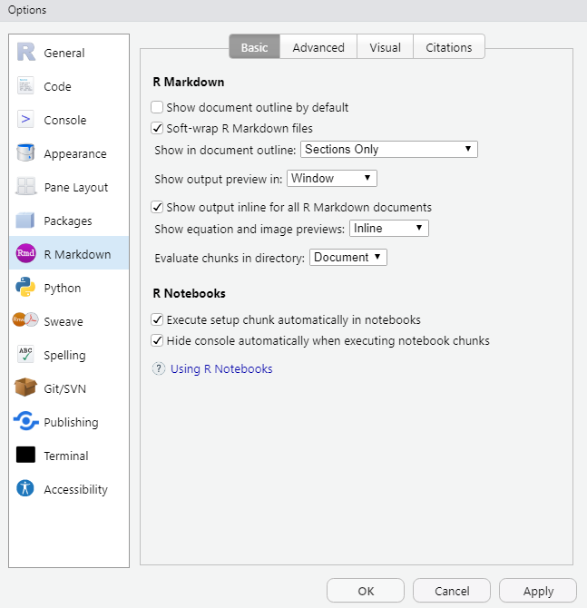
RStudio offers various functions that facilitate working with .Rmd documents, which can be controlled at two locations:
- global settings that apply to all markdown projects, located at:
Tools -> Global Options -> R Markdown
RStudio — R Markdown Options
RStudio offers various functions that facilitate working with .Rmd documents, which can be controlled at two* locations:
- global settings that apply to all markdown projects, located at:
Tools -> Global Options -> R Markdown
- project settings that apply to a given markdown project, located at:
Tools -> Project Options -> R Markdown
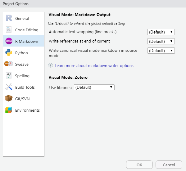
* Some settings become available on the document toolbar as well, only when an .Rmd document is open. We will cover the document toolbar later on in the workshop. All settings can stay as they are — for now.
R Packages — Install from within RStudio
install.packages(c("rmarkdown", "tinytex", "dplyr", "stargazer", "ggplot2"))tinytex::install_tinytex()R Packages — Install from within RStudio
install.packages(c("rmarkdown", "tinytex", "dplyr", "stargazer", "ggplot2"))tinytex::install_tinytex()rmarkdown(Allaire, Xie, McPherson, Luraschi, Ushey, Atkins, Wickham, Cheng, Chang, and Iannone, 2022), for automating the process of converting R Markdown documents into other formats
R Packages — Install from within RStudio
install.packages(c("rmarkdown", "tinytex", "dplyr", "stargazer", "ggplot2"))tinytex::install_tinytex()rmarkdown(Allaire, Xie, McPherson, et al., 2022), for automating the process of converting R Markdown documents into other formatstinytex(Xie, 2022c), for PDF outputs- requires an additional step to install
- alternative: a TeX/LaTeX system installed on your computer
R Packages — Install from within RStudio
install.packages(c("rmarkdown", "tinytex", "dplyr", "stargazer", "ggplot2"))tinytex::install_tinytex()dplyr(Wickham, François, Henry, and Müller, 2022), for data manipulation- popular alternative: e.g.,
base(R Core Team, 2022),data.table(Dowle and Srinivasan, 2021)
- popular alternative: e.g.,
R Packages — Install from within RStudio
install.packages(c("rmarkdown", "tinytex", "dplyr", "stargazer", "ggplot2"))tinytex::install_tinytex()dplyr(Wickham, François, Henry, et al., 2022), for data manipulation- popular alternative: e.g.,
base(R Core Team, 2022),data.table(Dowle and Srinivasan, 2021)
- popular alternative: e.g.,
stargazer(Hlavac, 2022), for tables- popular alternatives:
knitr(Xie, 2022b),kableExtra(Zhu, 2021),huxtable(Hugh-Jones, 2021)
- popular alternatives:
ggplot2, for figures- popular alternatives:
base(R Core Team, 2022),plotly(Sievert, Parmer, Hocking, Chamberlain, Ram, Corvellec, and Despouy, 2021)
- popular alternatives:
R Markdown Cheat Sheet — Download from the Internet
Downloading process can be initiated from within RStudio
- follow from the RStudio menu
Help -> Cheatsheets -> R Markdown Cheat Sheet
Other Resources*
Pandoc User's Guide
- available at https://pandoc.org/MANUAL.html
R Markdown: The Definitive Guide (Xie, Allaire, and Grolemund, 2018)
- open access at https://bookdown.org/yihui/rmarkdown
R for Data Science (Wickham and Grolemund, 2021)
- open access at https://r4ds.had.co.nz
* During the workshop, R Markdown Cheat Sheet is likely to be more helpful than these resources, which I recommend to be consulted after the workshop.
R Markdown Document — Create from within RStudio
- Create a new R Markdown document from the RStudio menu:*
File -> New File -> R Markdown -> OK
- Save your new document:**
File -> Save
Observe that
- the document has been saved to your working directory, and
- it has the .Rmd extension
* This is for demonstration purposes only. Otherwise, we will work with journals.Rmd, which you have already downloaded, to save time.
** Alternatively, use the Save button or the keyboard shortcut (e.g., Ctrl + S on Windows). For shortcuts, follow Tools -> Keyboard Shortcuts Help or Tools -> Modify Keyboard Shortcuts....
R Markdown Document — Components
Observe also that the document has three components
- YAML

R Markdown Document — Components
Observe also that the document has three components
- YAML
- text
R Markdown Document — Components
Observe also that the document has three components
- YAML
- text
- code chunks
R Markdown Document — Document Toolbar
Observe also that the document toolbar offers extended tools for .Rmd documents

These include, most impotantly,
- the
 button to compile .Rmd documents
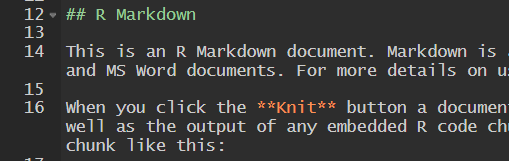
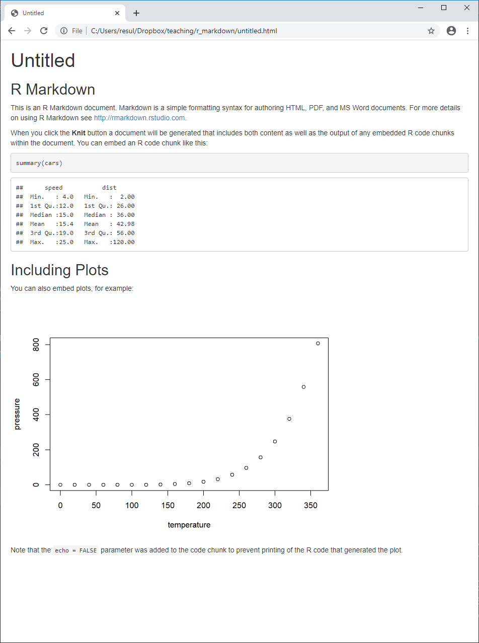
R Markdown Document — Compile
Click the
Knitbutton to compile your .Rmd document, and observe that- the output document has the same name as your .Rmd document
You may want to delete these newly created files, as we will work with
journals.Rmdinstead to save time.
R Markdown Document — Compilation Process
When you
Knit, the following happens:.Rmd --knitr--> .md --pandoc--> outputknitr* executes the code if there is any, converts the resulting document from .Rmd (R Markdown) into .md (Markdown)pandoc** transforms the .md document into your preferred output format(s)- e.g., HTML, LaTeX, PDF, Word
This process is automated by the
rmarkdownpackage
* If you had not already have the knitr package, it would have been installed together with the rmarkdown package.
** RStudio comes with a copy of pandoc (http://pandoc.org), which is not an R package, so that you do not have to install it separately.
R Markdown Document — Notes
Behind the scenes, each .Rmd file is compiled in its own session, and therefore
- the code needs to stand alone, for reproducibility reasons
- e.g., if you load a package in the Console, it will not be available to a given .Rmd file — even in the same R session
R Markdown Document — Notes
Behind the scenes, each .Rmd file is compiled in its own session, and therefore
- the code needs to stand alone, for reproducibility reasons
- e.g., if you load a package in the Console, it will not be available to a given .Rmd file — even in the same R session
R Markdown can produce more than documents,* including
- presentations, again with
rmarkdown - books, with
bookdown(Xie, 2022a) - websites, with
blogdown(Xie, Dervieux, and Presmanes Hill, 2022)
- presentations, again with
* Here we will focus on research papers only. In a separate workshop, I teach how to create professional websites with R Blogdown.
YAML — Overview
.Rmd documents start* with YAML
- includes the metadata variables
- e.g., title, output format
- e.g., title, output format
- written between a pair of three hyphens -
---title: output:---* Technically, we can place YAML anywhere in a .Rmd document. However, it is a good practice to start with YAML so that the metadata is easly accessbile.
YAML — Variables
titleandoutputare the basic variables of YAML- variable names are typed in lower case, followed by a colon :
- the list of available variables, as well as options and sub-options for these variables, depends on the output format
- Pandoc User's Guide provides a comprehensive documentation
- R Markdown Cheat Sheet provides a helpful list
- variable names are typed in lower case, followed by a colon :
Typical YAML variables for an research paper are as follows:
---title: author: date: bibliography: csl: output: ---YAML — Variables
Variables can take strings
---title: "Journals: Random Words With Random Data"output:---YAML — Variables
Variables can take strings, options
---title: "Journals: Random Words With Random Data" output: pdf_document---YAML — Variables
Variables can take strings, options, sub-options
---title: "Journals: Random Words With Random Data" output: pdf_document: keep_tex: true---YAML — Variables
Variables can take strings, options, sub-options, and code
---title: "Journals: Random Words With Random Data" output: pdf_document: keep_tex: truedate: "`r format(Sys.Date(), '%d %B %Y')`"---YAML — Variables — Output Formats
Documents as output formats include
- HTML
---title: "Journals: Random Words With Random Data" output: html_document---
YAML — Variables — Output Formats
Documents as output formats include
- HTML
- LaTeX
---title: "Journals: Random Words With Random Data" output: latex_document---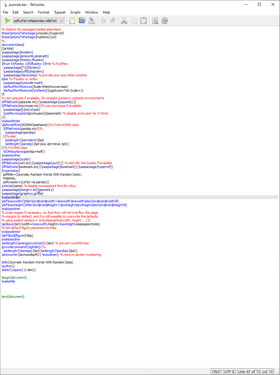
YAML — Variables — Output Formats
Documents as output formats include
- HTML
- LaTeX
---title: "Journals: Random Words With Random Data" output: pdf_document---
YAML — Variables — Output Formats
Documents as output formats include
- HTML
- LaTeX
- Word
---title: "Journals: Random Words With Random Data" output: word_document---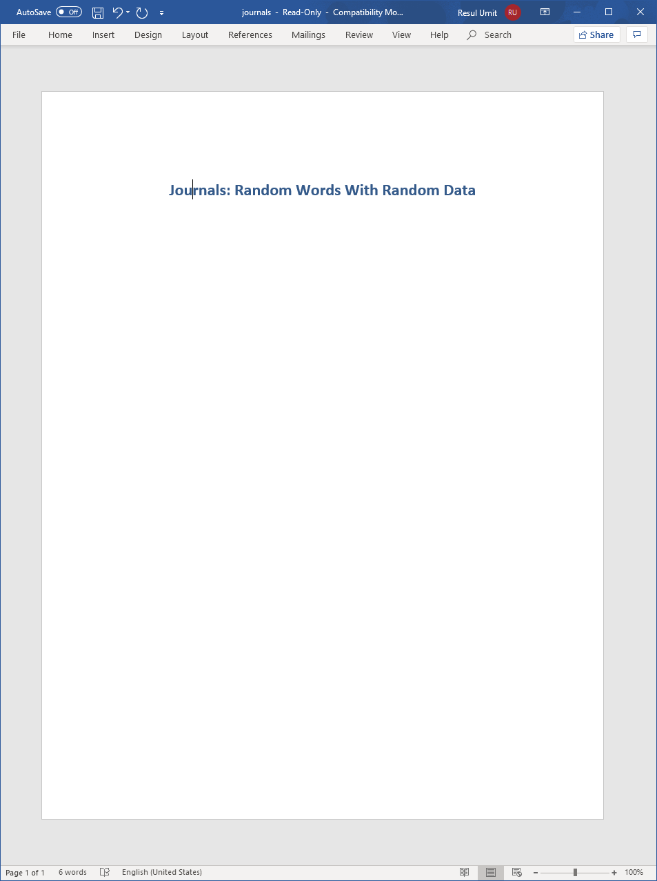
YAML — Variables — Output Formats
Documents as output formats
html_documentlatex_documentpdf_document*word_documentgithub_documentmd_documentodt_documentrtf_document
Presentations as output formats
beamer_presentationiosslides_presentationpowerpoint_presentationslidy_presentation
* For reasons of simplicity, this workshop focuses on LaTex and/or PDF outputs. Different output formats have slightly different customisations. See Pandoc User's Guide and/or R Markdown Cheat Sheet.
YAML — Strings
Strings with special characters, such as colon, require quotation marks — single ' or double "
---title: "Journals: Random Words With Random Data"output: pdf_document ---
YAML — Strings
Quotation marks are optional for strings without special characters
---title: "Journals: Random Words With Random Data" subtitle: A Mock Paper for an R Markdown Workshopauthor: Jane Doedate: 4 March 2020output: pdf_document ---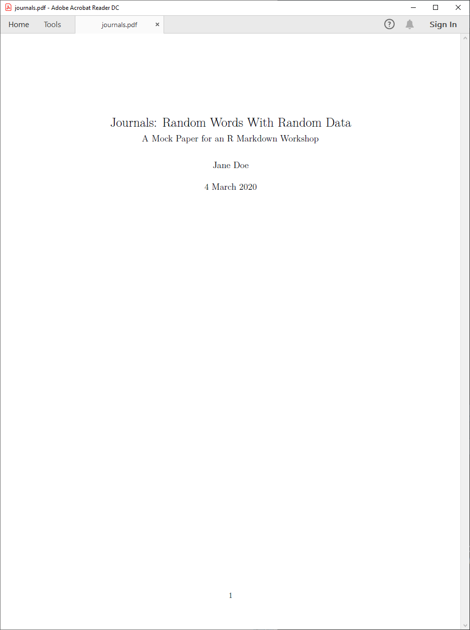
YAML — Strings — Footnotes
The syntax ^[footnotes_go_here] adds footnotes to strings
---title: "Journals: Random Words With Random Data^[Preliminary draft. Please do not cite or circulate without permission from the author.]"subtitle: A Mock Paper for an R Markdown Workshopauthor: "Jane Doe^[Department of Science, University of Random. Email: jane.doe@random.edu. Website: http://www.janedoe.com.]"date: 4 March 2020 output: pdf_document ---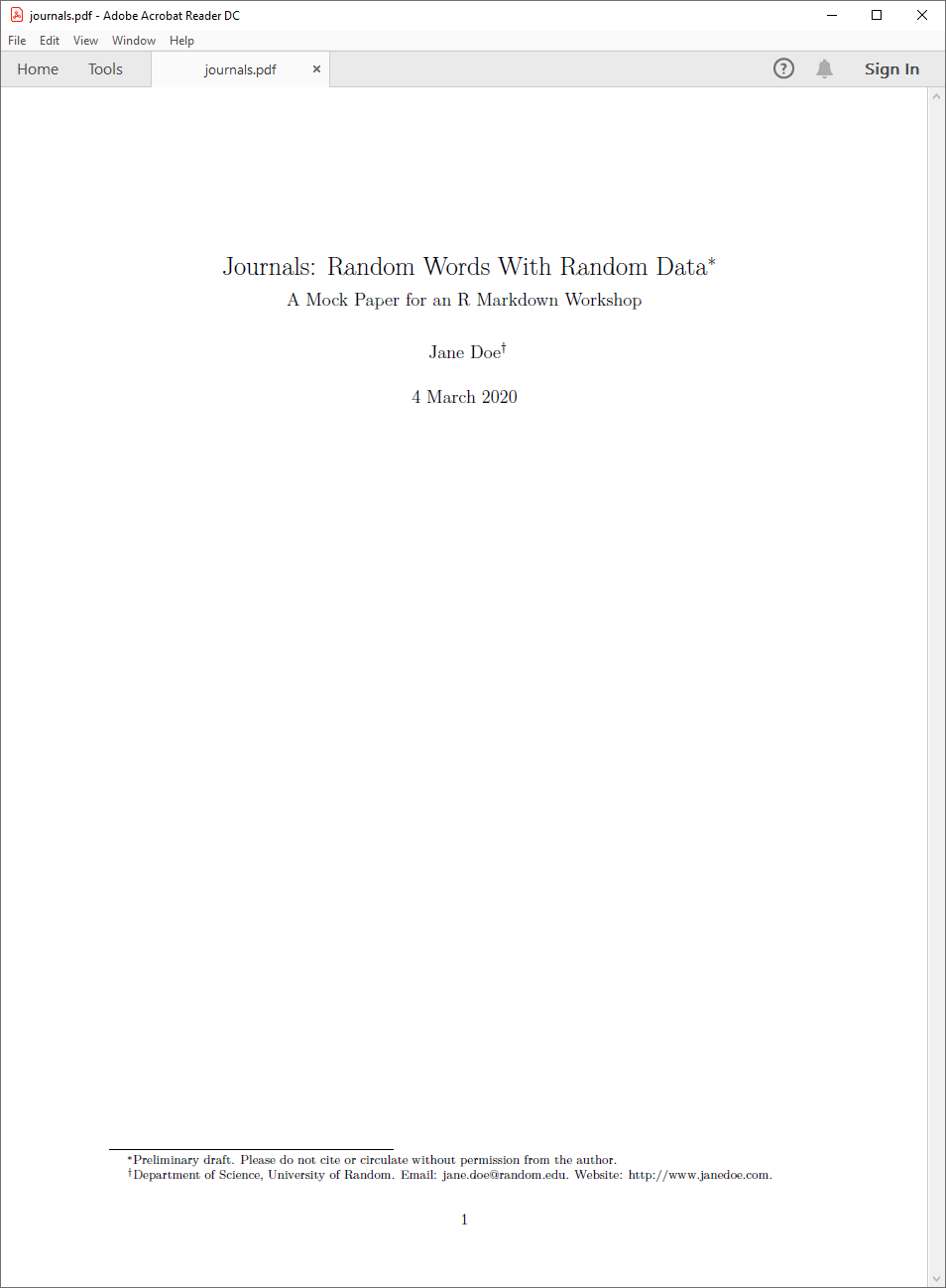
YAML — Strings — External Files
The bibliography and csl variables take strings as well
---title: "Journals: Random Words With Random Data^[Preliminary draft. Please do not cite or circulate without permission from the author.]"subtitle: A Mock Paper for an R Markdown Workshopauthor: "Jane Doe^[Department of Science, University of Random. Email: jane.doe@random.edu. Website: http://www.janedoe.com.]" date: 4 March 2020 bibliography: references.bibcsl: apa_7th.csloutput: pdf_document ---YAML — Strings — External Files
The strings for external files indicate (a) where the files are located and (b) how they are named
---...bibliography: references/ref_library.bib csl: "../../styles/chicago_manual_17.csl"...---YAML — Strings — External Files
The strings for external files indicate (a) where the files are located and (b) how they are named
---...bibliography: references/ref_library.bib csl: "../../styles/chicago_manual_17.csl"...---Notice that
the locations above are specified as relative to the working directory
- the former (references) is a sub-directory, or folder, one level down while the latter (styles) is two levels up
for reproducibility reasons, hard-coded stings should be avoided
- e.g.,
"C:/Users/resulumit/Dropbox/styles/chicago_manual_17.csl"
- e.g.,
YAML — Strings — External Files
The strings indicate (a) where the files are located and (b) how they are named
---...bibliography: references/ref_library.bib csl: "../../styles/chicago_manual_17.csl"...---YAML — Options and Sub-Options
Options can have sub-options
---title: "Journals: Random Words With Random Data^[Preliminary draft. Please do not cite or circulate without permission from the author.]"subtitle: A Mock Paper for an R Markdown Workshopauthor: "Jane Doe^[Department of Science, University of Random. Email: jane.doe@random.edu. Website: http://www.janedoe.com.]"date: 4 March 2020 bibliography: references.bibcsl: apa_7th.csl output: pdf_document: keep_tex: true---
YAML — Options and Sub-Options
Options can have sub-options
---title: "Journals: Random Words With Random Data^[Preliminary draft. Please do not cite or circulate without permission from the author.]"subtitle: A Mock Paper for an R Markdown Workshopauthor: "Jane Doe^[Department of Science, University of Random. Email: jane.doe@random.edu. Website: http://www.janedoe.com.]" date: 4 March 2020 bibliography: references.bibcsl: apa_7th.csl output: pdf_document: keep_tex: true---Notice that
this specific setting, highlighted, will create multiple outputs
- a LaTeX and a PDF document
all but the last option (i.e.,
true) takes a colonoptions and sub-options (except the last option, again) are stepwise indented
- exactly with four spaces
- the alignment between the colons for
pdf_documentandkeep_texis coincidental
YAML — R Code
Variables can take code as well
---title: "Journals: Random Words With Random Data^[Preliminary draft. Please do not cite or circulate without permission from the author.]"subtitle: A Mock Paper for an R Markdown Workshopauthor: "Jane Doe^[Department of Science, University of Random. Email: jane.doe@random.edu. Website: http://www.janedoe.com.]"date: "`r format(Sys.Date(), '%d %B %Y')`"bibliography: references.bibcsl: apa_7th.csl output: pdf_document---
YAML — R Code
Variables can take code as well
---title: "Journals: Random Words With Random Data^[Preliminary draft. Please do not cite or circulate without permission from the author.]"subtitle: A Mock Paper for an R Markdown Workshopauthor: "Jane Doe^[Department of Science, University of Random. Email: jane.doe@random.edu. Website: http://www.janedoe.com.]"date: "`r format(Sys.Date(), '%d %B %Y')`"bibliography: references.bibcsl: apa_7th.csl output: pdf_document---Notice that
such codes can be particularly useful for variables
- that need frequent updates
- and that can be automatically updated
- e.g.,
date
- e.g.,
there are quotation marks around the code
we will cover codes in .Rmd documents later on in the workshop
YAML — R Code
Code and text can be combined in a string
---title: "Journals: Random Words With Random Data^[Preliminary draft. Please do not cite or circulate without permission from the author.]"subtitle: A Mock Paper for an R Markdown Workshopauthor: "Jane Doe^[Department of Science, University of Random. Email: jane.doe@random.edu. Website: http://www.janedoe.com.]"date: "First version: 4 March 2020. This version: `r format(Sys.Date(), '%d %B %Y')`."bibliography: references.bibcsl: apa_7th.csl output: pdf_document---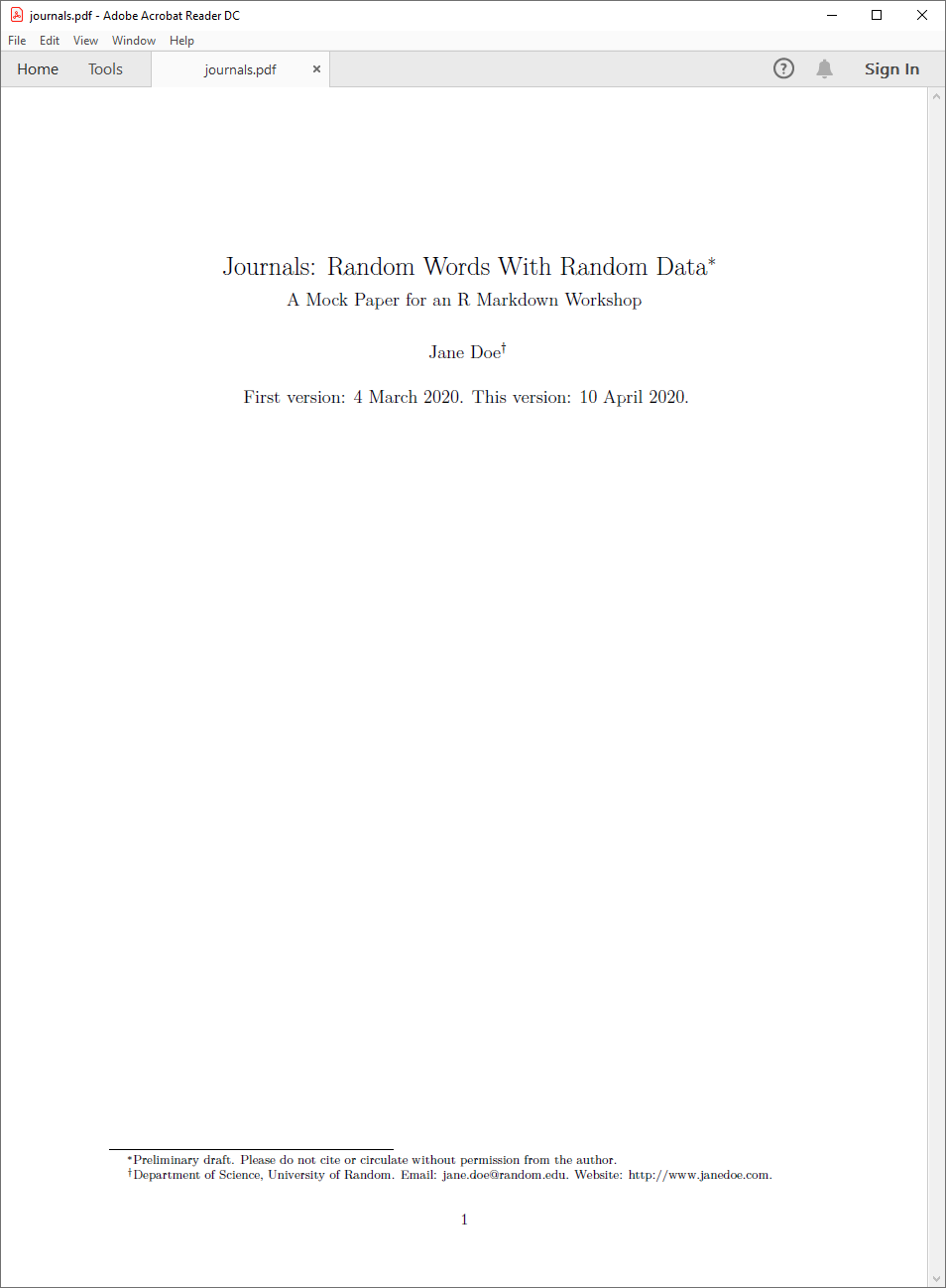
YAML — Some Further Settings for PDF Outputs
fontsize- the default is
10pt - the other options are
11ptand12pt
- the default is
linkcolor,urlcolor,citecolor- the default is the colour of the text
- the other options are white, red, green, blue, cyan, magenta, yellow
link-citations- the default is
no - the other option is
yes— a click on an citation will take the screen to the relevant entry in the list of references
- the default is
Exercises — 1–4
1) Open journals.Rmd and fill in the YAML variables for the mock paper
- take cues from
reproduce_this.pdfand/or the slides
2) Add and set one of the variables mentioned as further settings for PDF outputs above
- i.e.,
fontsize,linkcolor,urlcolor,citecolor,link-citations
3) Add and set a completely new variable not covered so far
- see, for example, the R Markdown Cheat Sheet
4) Knit your journals.Rmd
- observe the outcome
10:00
Syntax — Overview
There are not one, but several different versions of Markdown
- e.g., Pandoc, MultiMarkdown, CommonMark
- each might implement the same things (e.g., citations) slightly differently, and each might offer unique functionalities
R Markdown follows the syntax in Pandoc's Markdown
- for the complete rules of the syntax, see Pandoc User's Guide
- for a useful summary of the syntax, see the R Markdown Cheat Sheet
Syntax — Lines
Multiple spaces on a given line are reduced to one
This is a sentence followed by four spaces. This is another sentence on the same line.This is a sentence followed by four spaces. This is another sentence on the same line.
Line endings with fewer than two spaces are ignored
This is a sentence followed by one space.This is another sentence on a new line.This is a sentence followed by one space. This is another sentence on a new line.
Syntax — Hard Breaks
Two or more spaces at the end of lines introduce hard breaks, forcing a new line
This is a sentence followed by two spaces. This is another sentence on a new line.This is a sentence followed by two spaces.
This is another sentence on a new line.
Syntax — Line Blocks
Spaces on lines that start with a vertical line | are kept
| a one-space indent| a five-space indent| a ten-space indent a one-space indent
a five-space indent
a ten-space indent
Syntax — Block Quotes
Lines starting with the greater-than sign > introduce block quotes*
> In God, we trust. All others must bring data. >> --- Anonymous In God, we trust. All others must bring data.
— Anonymous
* Notice that three hyphens grouped together introduce an em-dash. Dashes are covered later on in the workshop.
Syntax — Paragraphs
One or more* blank lines introduce a new paragraph
This is the first sentence of a paragraph as it is preceded by a blank line. This is the second sentence of that paragraph, which is followed by a blank line. This is the first sentence of a *new paragraph* as it is preceded by a blank line. This is the second sentence of that paragraph, which is followed by a blank line.This is the first sentence of a paragraph as it is preceded by a blank line. This is the second sentence of that paragraph, which is followed by a blank line.
This is the first sentence of a new paragraph as it is preceded by a blank line. This is the second sentence of that paragraph, which is followed by a blank line.
* Multiple blank lines between paragraphs reduce to one.
Syntax — Comments
Text with the syntax <!--comments --> is omitted from output
<!-- This paragraph needs re-writing -->This is the first sentence of a paragraph as it is preceded by a blank line. This is the second sentence of that paragraph, which is followed by a blank line. This is the first sentence of a new paragraph <!-- I've removed italics --> as it is preceded by a blank line. This is the second sentence of that paragraph, which is followed by a blank line.This is the first sentence of a paragraph as it is preceded by a blank line. This is the second sentence of that paragraph, which is followed by a blank line.
This is the first sentence of a new paragraph as it is preceded by a blank line. This is the second sentence of that paragraph, which is followed by a blank line.
Exercises — 5–6
5) Hard Breaks
- see
reproduce_this.pdf, page 1 - apply in
journals.Rmd, paragraph 1
6) Line Blocks / Block Quotes
- see
reproduce_this.pdf: page 1 - apply in
journals.Rmd: block quote, between paragraphs 1 and 2 - see
reproduce_this.pdf: page 5 - apply in
journals.Rmd: hypothesis 1, between paragraphs 14 and 15; hypothesis 2, between paragraphs 16 and 17
05:00
Syntax — Headers
The number sign # introduces headers; lower levels are created with additional signs — up to total five levels
# Introduction becomes
Introduction
## 1. Introduction becomes
1. Introduction
### 3.1 Introduction becomes
3.1 Introduction
#### Introduction becomes
Introduction
##### Introduction becomes
Introduction
Syntax — Emphases
A pair of single asterisk * or underscores _ introduces italics
*italics* becomes italics
_italics_ becomes italics as well
A pair of double asterisk or underscores introduces bold
**bold** becomes bold
__bold__ becomes bold as well
These two rules can be combined
**_bolditalics_** becomes bolditalics
_**bolditalics**_ becomes bolditalics as well
Syntax — Strikethrough
A pair of double tildes ~ introduces strikethrough
~~strikethrough~~ becomes strikethrough
Strikethrough can be combined with italics or bold
**~~strikebold~~** or __~~strikebold~~__, they both become strikebold
~~**strikebold**~~ or ~~__strikebold__~~, they both become strikebold as well
*~~strikeitalitcs~~* or _~~strikeitalitcs~~_, they both become strikeitalitcs
~~*strikeitalitcs*~~ or ~~_strikeitalitcs_~~, they both become strikeitalitcs as well
Exercises — 7–8
7) Headers
- see
reproduce_this.pdf: pages 1 to 11- 10 headers, Abstract to References
- 10 headers, Abstract to References
- apply in
journals.Rmd
8) Emphases
- see
reproduce_this.pdf: pages 1 and 2- bold and italics
- bold and italics
- apply in
journals.Rmd: paragraph 2
03:00
Syntax — Links — Internal*
You can link text to section headers in the same document
[Conclusion](#conclusion) becomes Conclusion, and a click takes the screen to that section
Multi-word headers need hyphenation
[Literature Review](#literature-review) becomes Literature Review, and it works only if the second part is hyphenated
* The links to references, figures, and tables are covered later on in the workshop.
Syntax — Links — External
You can link text to URLs
[visit my website](https://resulumit.com/) becomes visit my website
[https://resulumit.com](https://resulumit.com/) becomes https://resulumit.com
<https://resulumit.com> becomes https://resulumit.com as well
Syntax — Links — External
You can link text to URLs
[visit my website](https://resulumit.com/) becomes visit my website
[https://resulumit.com](https://resulumit.com/) becomes https://resulumit.com
<https://resulumit.com> becomes https://resulumit.com as well
You can also link text to an email address
[email me](mailto:resuluy@uio.no)* becomes email me
<resuluy@uio.no> becomes resuluy@uio.no
* Notice the prefix mailto: in the syntax.
Exercises — 9–10
9) Links — Internal
- see
reproduce_this.pdf: page 2- the link to the Literature Review section
- the link to the Literature Review section
- apply in
journals.Rmd: paragraph 4
10) Links — External
- see
reproduce_this.pdf: page 1- email and website links in one of the footnotes
- email and website links in one of the footnotes
- apply in
journals.Rmd: title page items
03:00
Syntax — Equations
Inline equations go between a pair of single dollar signs $ — with no space between the signs and the equation itself
$E = mc^{2}$ becomes E = mc2
Syntax — Equations
Inline equations go between a pair of single dollar signs $ — with no space between the signs and the equation itself
$E = mc^{2}$ becomes E = mc2
Block equations go in between a pair of double dollar signs — with or without spaces, it works
$$ E = mc^{2}$$ becomes
$$E = mc_{2}$$ becomes
Syntax — Footnotes — Inline Notes
For inline footnotes, use the ^[footnote] syntax
Jane Doe^[Corresponding author.] becomes Jane Doe1
1 Corresponding author.
Syntax — Footnotes — Inline Notes
For inline footnotes, use the ^[footnote] syntax
Jane Doe^[Corresponding author.] becomes Jane Doe1
1 Corresponding author.
Notice that
- the caret sign ^ comes before the left square bracket [
- this syntax works in YAML as well as in text
- footnotes in YAML get symbols, in text they get numbers
Syntax — Footnotes — Notes with Identifiers
An alternative is to use the [^identifier] syntax, with identifiers defined elsewhere in the same document
Dr Doe holds a PhD in rock science.[^defence_date][^defence_date]: She defended her thesis in 2017.Dr Doe holds a PhD in rock science.1
1 She defended her thesis in 2017.
Notice that
- the caret sign comes after the left square bracket
- this syntax works in text, but not in YAML
Exercises — 11–12
11) Equations
- see
reproduce_this.pdf: page 7 - apply in
journals.Rmd: paragraph 22; block equation, between paragraphs 22 and 23
12) Footnotes
- see
reproduce_this.pdf: page 2 - apply in
journals.Rmd: paragraph 3
03:00
Syntax — Lists
Lines starting with asterisk * as well as plus + or minus − signs introduce lists
- books- articles- reports- books
- articles
- reports
Syntax — Lists — Nesting
Lists can be nested within each other, with indentation
+ books+ articles - published - under review + revised and resubmitted - work in progress- books
- articles
- published
- under review
- revised and resubmitted
- work in progress
Syntax — Lists — Numbering
List items can be numbered
1. books2. articles - published - under review + revised and resubmitted - work in progress- books
- articles
- published
- under review
- revised and resubmitted
- work in progress
Syntax — Dashes
Two hyphens grouped together introduce an en-dash
‐‐ becomes –
Three hyphens grouped together introduce an em-dash
‐‐‐ becomes —
Syntax — Subscripts and Superscripts
A pair of tildes introduces subscript
CO~2~ becomes CO2
A pair of carets introduces superscript
R^2^ becomes R2
Syntax — Subscripts and Superscripts
A pair of tildes introduces subscript
CO~2~ becomes CO2
A pair of carets introduces subscript
R^2^ becomes R2
Notice that
- the syntax here (Markdown-based) is different than the one for equations (LaTeX-based)
- e.g., R^2^ versus mc^{2}
Exercises — 13–15
13) Lists
- see
reproduce_this.pdf: page 3 - apply in
journals.Rmd: list, between paragraphs 10 and 11
14) Dashes
- see
reproduce_this.pdf: page 2 - apply in
journals.Rmd: paragraph 6
15) Subscripts and Superscripts
- see
reproduce_this.pdf: page 2 - apply in
journals.Rmd: paragraph 5
03:00
References — Bibliography Database
References are defined in .bib files
- they follow the BibTeX format
pandoclooks for a .bib file, and for the definitions therein, to process citations- .bib files are specified with the
bibliographyvariable in YAML
- .bib files are specified with the
pandoccan process a citation only if there is a linked entry in the .bib file- but not all entries have to be cited
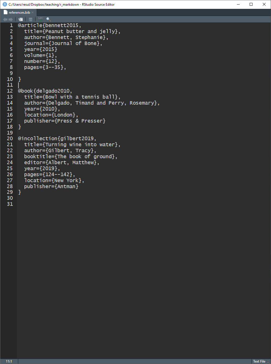
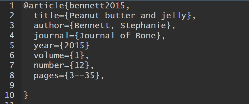
References — Bibliography Database — Entries
A BibTeX entry consists of three elements
- a type
- e.g.,
@article
- e.g.,
- a citation-key
- e.g.,
bennett2015
- e.g.,
- a number of tags
- e.g.,
title,author
- e.g.,
- a type
Different tags are available for different reference types
- some tags are required, others are optional
References — Bibliography Database — Entries
One could create entries by hand
- requires knowing the BibTeX format, entry types, tags, and related information about references to be cited
- neither efficient nor necessary
A good alternative is to use
Google Scholar, which provides BibTeX entries- follow
cite -> BibTexand copy - paste into .bib, edit if necessary, and save
- follow
- Some publishers and journals provide BibTeX entries on their website as well
References — Style
Reference styles are defined in .csl files
- files for different styles (e.g., APA) are available at https://www.zotero.org/styles
pandoclooks for a .csl file, and for the styles therein, to style citations and references- .csl files are specified with the
cslvariable in YAML - if unspecified, it uses a Chicago author-date format
- .csl files are specified with the
.csl files affect the style only in outputs
- no matter which the style is used, the citation syntax in .Rmd documents remains the same
References — In-text Citation Syntax — Author-Date Styles*
All citations keys take the 'at' sign @ while square brackets and/or minus signs introduce variation
[@bennett2015] becomes (Bennett, 2015)
@bennett2015 becomes Bennett (2015)
[-@bennett2015] becomes (2015)
-@bennett2015 becomes 2015
[@bennett2015 35] becomes (Bennett, 2015, p. 35)
[@bennett2015 33-35] becomes (Bennett, 2015, pp. 33–35)
[@bennett2015, ch. 1] becomes (Bennett, 2015, ch. 1)
[@bennett2015; @gilbert2019] becomes (Bennett, 2015; Gilbert, 2019)
[see @bennett2015, for details] becomes (see Bennett, 2015, for details)
@bennett2015 [33-35] becomes Bennett (2015, pp. 33–35)
* Specifically, the outputs on this slide are formatted according to the APA 7th edition.
References — In-text Citation Syntax — Numerical Styles
All citations keys take the 'at' sign @
A clever sentence.[@bennett2015] becomes A clever sentence.[1] in certain numerical sytles
A clever sentence.[@bennett2015; @gilbert2019] becomes A clever sentence.[1,2]
References — In-text Citation Syntax — Numerical Styles
All citations keys take the 'at' sign @
A clever sentence.[@bennett2015] becomes A clever sentence.[1] in certain numerical sytles
A clever sentence.[@bennett2015; @gilbert2019] becomes A clever sentence.[1,2]
Individual styles may or may not use additional information, such as page numbers
A clever sentence.[@bennett2015 35] might become A clever sentence.[1] as well
Individual styles may or may not be sensitive to variation, such as square brackets
A clever sentence. @bennett2015 might become A clever sentence.[1] as well
Citations — Reference List
The list of references appears after the last line of the output document, with no section header
- so that you can choose the header yourself, by ending .Rmd documents with a header of your choice
This is the last sentence of an APA style manuscript.## ReferencesThis is the last sentence of an APA style manuscript.
References
Bennett, S. (2015). Peanut butter and jelly. Journal of Bone, 1(12), 3–35.
Gilbert, T. (2019). Turning wine into water. In M. Albert (Ed.), The book of ground (pp. 124–142). Antman.
References — Internal Links
For internal links from in-text citations to the reference list, set link-citations: yes in YAML
- a click on these links takes the screen to the relevant entry in the list
- the
linkcolorvariable make these links explicit- setting this is not necessary for the links to work — the default is black
---...bibliography: references.bibcsl: apa_7th.csllink-citations: yeslinkcolor: blue...---Exercises — 16–19
16) Add an entry to references.bib for the following book
- R Markdown: The Definitive Guide by Xie and co-authors
17) Reproduce the citations and reference list in the mock paper
- see
reproduce_this.pdf: pages 3 and 11 - apply in
journals.Rmd: paragraph 7 to 9
18) Change the reference style
- download the .csl file for your favourite style from https://www.zotero.org/styles
- put it into your working directory
- update the YAML variable
19) Link the citations to the reference list
07:30
Code, in and outside Chunks
Code — Overview
Most codes go inside code chunks
- e.g., code that imports and cleans data, and/or produces tables and/or figures
```{r}df <- read.csv("rmd_workshop_files/images_data/journals.csv") %>% mutate(age = 2020 - since, english = factor(english), subfield = factor(subfield))```Codes can also go in line with text
- e.g., code that results in a single statistic
The average H5 Index for the journals in the dataset is `r mean(df$h5_index)`.Code Chunks — Overview
Code chunks are delimited spaces between a pair of three backticks `
- placed on their own lines in .Rmd documents, separate from text
- their output, if there is any, appear in the output document
- at about the same place as the chunk
- might float around text to avoid breaking across pages
``````Code Chunks — Overview
Code chunks are delimited spaces between a pair of three backticks `
- placed on their own lines in .Rmd documents, separate from text
- their output, if there is any, appear in the output document
- at about the same place as the chunk
- might float around text to avoid breaking across pages
On the same line with the first delimiter, and in curly brackets {, code chunks take
- a languge engine
```{r}```Code Chunks — Overview
Code chunks are delimited spaces between a pair of three backticks `
- placed on their own lines in .Rmd documents, separate from text
- their output, if there is any, appear in the output document
- at about the same place as the chunk
- might float around text to avoid breaking across pages
On the same line with the first delimiter, and in curly brackets {, code chunks take
- a language engine
- a label
```{r, setup}```Code Chunks — Overview
Code chunks are delimited spaces between a pair of three backticks `
- placed on their own lines in .Rmd documents, separate from text
- their output, if there is any, appear in the output document
- at about the same place as the chunk
- might float around text to avoid breaking across pages
On the same line with the first delimiter, and in curly brackets {, code chunks take
- a language engine
- a label
- one or more options
```{r, setup, echo=FALSE}```Code Chunks — Lenguage Engines
The first item in code chunks indicates the engine to run the code
```{r}```Note that
indicating an engine for each chunk is a must
- otherwise, any code* in these chunks cannot be executed
ris the specified engine, indicating that the code in the chunk above should be run by R- it could have been
python, which we will not cover in this workshop
- it could have been
* The above chunk has no code — it is for demonstration only.
Code Chunks — Labels
It is recommended, but optional, to label the code chunks
```{r, data_import}df <- read_csv("data/journals.csv")```Note that
labels are written after the language engine, separated by a comma
- in the example above, the chunk is labelled as
data_import
- in the example above, the chunk is labelled as
chunks without labels are otherwise automatically numbered
- specifying informative labels can be helpful for, e.g., navigating through error messages
duplicate labels lead to errors during compilation
Code Chunks — Options
Code chunks can take further options
```{r, setup, include=FALSE}```Note that
in the example above, the
includeoption is set toFALSE- with this option and value, nothing from this chunk will be included in the output document
The complete list of options is available at https://yihui.org/knitr/options
- R Markdown Cheat Sheet provides a helpful list as well
leaving spaces around the equal sign =, between option tags and values, should be avoided
- such spaces might lead to errors
Code Chunks — Options — Alternative Syntax
Options can be specified inside code chunks as well, after a number sign and a vertical line #|
- therefore the following chunks have the same function
```{r, echo=FALSE, eval=TRUE}``````{r}#| echo = FALSE, eval = TRUE``````{r}#| echo = FALSE#| eval = TRUE```Code Chunks — Options — Defaults
Options have default values
- e.g., for
echo, the default isTRUEecho: should the source code printed in the output?TRUE: yes it should
- therefore the following two chunks have the same function
```{r}``````{r, echo=TRUE}```Code Chunks — Options — Defaults
This chunk prints two things in the output document — (a) the code and (b) the head of the data frame
```{r}head(df)```head(df)
## name origin branch h5_index h5_median english subfield## 1 Journal of Bears Americas Physical 73 97 1 1## 2 Journal of Moon Asia Social 72 106 1 0## 3 Journal of Lumber Americas Physical 72 100 1 1## 4 Journal of Houses Europe Social 72 102 1 0## 5 Journal of Water Europe Social 70 100 1 0## 6 Journal of Jeans Americas Physical 69 101 1 1## issues age## 1 7 61## 2 6 64## 3 8 30## 4 8 38## 5 5 33## 6 5 64Code Chunks — Options — Examples
Setting echo=FALSE prevents the code from being displayed in the output document
```{r ... echo=FALSE}head(df)```This chunk therefore prints one thing in the output document — the head of the data frame
## name origin branch h5_index h5_median english subfield## 1 Journal of Bears Americas Physical 73 97 1 1## 2 Journal of Moon Asia Social 72 106 1 0## 3 Journal of Lumber Americas Physical 72 100 1 1## 4 Journal of Houses Europe Social 72 102 1 0## 5 Journal of Water Europe Social 70 100 1 0## 6 Journal of Jeans Americas Physical 69 101 1 1## issues age## 1 7 61## 2 6 64## 3 8 30## 4 8 38## 5 5 33## 6 5 64Code Chunks — Options — Examples
Prevent the result(s) of the source code from being displayed in the output document
```{r ... results="hide"}head(df)```This chunk therefore prints one thing in the output document — the source code
head(df)
Setting results="asis" passes the results as they are produced by the code — pandoc does not transform these. In creating tables for PDF output with the stargazer package, this option is a must.
Code Chunks — Options — Examples
Cache results for future compilations
```{r ... cache=TRUE}```Code Chunks — Options — Examples
Cache results for future compilations
```{r ... cache=TRUE}```Note that caching
is useful especially for chunks that take a long time to execute
- it can speed up the compilation process
avoids executing the chunks at every compilation
- unless the chunk is newly created or edited since the last cached compilation
creates a new folder in your working directory
- an alternative location can be specified with the
cache.pathoption
- an alternative location can be specified with the
Code Chunks — Options — Examples
Prevent R from running the code in the chunk altogether
```{r ... eval=FALSE}```Code Chunks — Options — Examples
Prevent R from running the code in the chunk altogether
```{r ... eval=FALSE}```Prevent messages and/or warnings from being displayed in the output
```{r ... error=FALSE, message=FALSE, warning=FALSE}```Code Chunks — Options — Examples
Define the actual dimensions of figures, in inches
```{r ... fig.height=6, fig.width=9}```Code Chunks — Options — Examples
Define the actual dimensions of figures, in inches
```{r ... fig.height=6, fig.width=9}```Define the size of figures as they appear in the output document, with out.width and/or out.height
```{r ... out.width="50%"}```Code Chunks — Options — Examples
Define the actual dimensions of figures, in inches
```{r ... fig.height=6, fig.width=9}```Define the size of figures as they appear in the output document, with out.width and/or out.height
```{r ... out.width="50%"}```Define the alignment of figures — left, right, or center
```{r ... fig.align="center"}```Code Chunks — Options — Examples
Define captions for figures
```{r ... fig.caption="A Scatter Plot"}```Code Chunks — Options — Examples
Define captions for figures
```{r ... fig.caption="A Scatter Plot"}```Set the resolution for figures
```{r ... dpi=300}```Code Chunks — Options — Examples
Define captions for figures
```{r ... fig.caption="A Scatter Plot"}```Set the resolution for figures
```{r ... dpi=300}```Set extra options, such as angle, that output format would accept for figures
```{r ... out.extra="angle=45"}```Code Chunks — The Setup Chunk
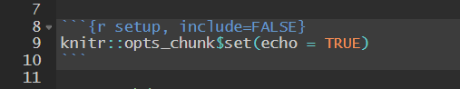
It is recommended to use the first code chunk for general setup, where you can
- define your own defaults for chunk options, with
knitr::opts_chunk$set()- avoids repeating chunk options
- avoids repeating chunk options
- load the necessary packages
- import raw data
```{r, setup, include=FALSE}# chunk option defaultsknitr::opts_chunk$set(echo=FALSE, message=FALSE)# packageslibrary(dplyr)library(ggplot2)library(stargazer)# datadf_raw <- read.csv("journals.csv")```Code Chunks — The Data Chunk
I recommend using the second chunk for the main operations* on raw data
- e.g., for data cleaning and other transformations
- some minor transformations could be left to lower chunks
- e.g., capitalizing variable names for figures
```{r, data, ...}df <- df_raw %>% mutate(subfield = as.factor(subfield), english = as.factor(english), age = 2020 - since) %>% select(-since)```* I will be using the pipe operator %>% and other functions from the dplyr package for such operations in the following slides.
Inline Code — Overview
Code can also be incorporated in text, with the `r ` syntax
- unlike chunks, these do not take options
- the output document will display the result of the code
- in the exact place of the source code
- in the exact place of the source code
- the result of the code will have the same formatting with the text
Inline Code — Examples
If we multiply _pi_ by 5, we get `r pi * 5`.If we multiply pi by 5, we get 15.7079633.
The average H5 Index for the journals in the dataset is `r mean(df$h5_index)`, which would round to `r round(mean(df$h5_index), digits = 1)`.The average H5 Index for the journals in the dataset is 26.3611366, which would round to 26.4.
__Only `r nrow(subset(df, english == 0))` journals__ in the dataset are published in a languageother than English.Only 113 journals in the dataset are published in a language other than English.
Exercises — 20–22
20) Setup Chunk
- introduce a setup chunk with one or more defaults chunk options, with
knitr::opts_chunk$set() - load the packages that we will need —
dplyr,ggplot2, andstargazer - import raw data
21) Data Chunk
- introduce a data chunk to transform
subfieldandenglishinto factors - create a new variable
age, based onsince - drop
sincefrom the data frame
22) Inline code
- see
reproduce_this.pdf: page 6- i.e., 1091 observations
- i.e., 1091 observations
- apply in
journals.Rmd: paragraph 21- hint: use the
nrowfunction
- hint: use the
07:30
Figures
Figures — Images — Markdown Syntax
The syntax  embeds images, and/or figures produced elsewhere,* into .Rmd documents
- similar to the link syntax, only this time it is preceded by an exclamation mark !
- goes outside code chunks, on a new line
- simple, but not very customisable
* Ideally, reproducible papers should produce their own images with data and code. However, there might be situations where this is not possible.
Figures — Images — Markdown Syntax

Figures — Images — Markdown Syntax
Figures are numbered automatically

Figures — Images — Markdown Syntax
The syntax can accept width or height attributes as follows
{ width=40% }
Figures — Images — knitr
The knitr package offers a capable alternative with the include_graphics() function
this goes inside code chunks
- use the function with the double-colon operator ::
- e.g.,
knitr::include_graphics("figure.extension")
- e.g.,
- use the function with the double-colon operator ::
this is more customisable, through the use of code chunks
- size is defined with the
out.widthorout.hightoptions- rather than
fig.heightand/orfig.width
- rather than
- size is defined with the
Figures — Images — knitr
The knitr package offers a capable alternative with the include_graphics() function
```{r, screenshot, echo=FALSE, fig.cap="A screenshot of the Google Scholar homepage."}knitr::include_graphics("../image/google_scholar.png")```
Figures — Images — knitr
Size is defined with the chunk options out.width or out.hight
```{r ... out.width="40%"}knitr::include_graphics("../image/google_scholar.png")```
Figures — Images — knitr
Most other chunk options are common with figures plotted within R Markdown, such as fig.align
```{r ... fig.align="center"}knitr::include_graphics("../image/google_scholar.png")```
Exercise
23) Images
- see
reproduce_this.pdf: figure 1 on page 10 - apply in
journals.Rmd: figure 1, between paragraphs 19 and 20
03:00
Figures — ggplot2 — Overview
A powerful package for visualising data
Used widely, not only by academics, but also by large corporations such as the New York Times
A huge amount is written on this package. See, for example,
- the package documentation
- this book by its creator Hadley Wickham
- this reference page
- this webinar by one of its authors, Thomas Lin Pedersen
- these extensions, maintained by the
ggplot2community
Among its alternatives are the
baseandplotlypackages
Figures — ggplot2 — Basics
1) The ggplot function and the data argument
- specify a data frame in the main
ggplotfunction
ggplot(data = df)Figures — ggplot2 — Basics
1) The ggplot function and the data argument
- specify a data frame in the main
ggplotfunction
ggplot(data = df)2) The mapping aesthetics, or aes; most importantly, the variable(s) that we want to plot
- specify as an additional argument in the same
ggplotfunction
ggplot(data = df, mapping = aes(x = h5_median, y = h5_index, color = subfield))Figures — ggplot2 — Basics
1) The ggplot function and the data argument
- specify a data frame in the main
ggplotfunction
ggplot(data = df)2) The mapping aesthetics, or aes; most importantly, the variable(s) that we want to plot
- specify as an additional argument in the same
ggplotfunction
ggplot(data = df, mapping = aes(x = h5_median, y = h5_index, color = subfield))3) The geometric objects, or geom; the visual representations
- specify, after a plus sign +, as an additional function
ggplot(data = df, mapping = aes(x = h5_median, y = h5_index, color = subfield)) + geom_point()Figures — ggplot2
Put the code in a chunk, and give it a caption
```{r, scatterplot, fig.cap = "A scatterplot of journal metrics."}ggplot(data = df, mapping = aes(x = h5_median, y = h5_index, color = subfield)) + geom_point()```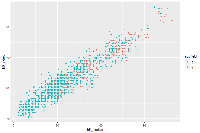
Figure 1. A scatterplot of journal metrics.
Figures — ggplot2
Add facets for subgroups, e.g., branch
```{r, scatterplot, fig.cap = "A scatterplot of journal metrics."}ggplot(data = df, mapping = aes(x = h5_median, y = h5_index, color = subfield)) + geom_point() + facet_wrap(. ~ branch)```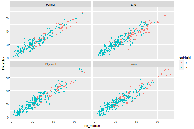
Figure 1. A scatterplot of journal metrics.
Figures — ggplot2
Scale the colour to improve the legend
```{r, scatterplot, fig.cap = "A scatterplot of journal metrics."}ggplot(data = df, mapping = aes(x = h5_median, y = h5_index, color = subfield)) + geom_point() + facet_wrap(. ~ branch) + scale_colour_discrete(name = "Journal Type", breaks = c(0, 1), labels = c("Generalist", "Subfield")) ```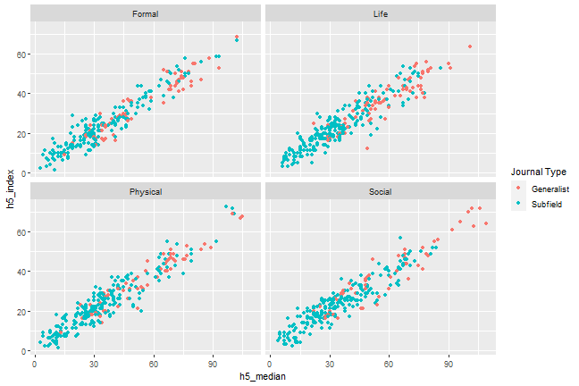
Figure 1. A scatterplot of journal metrics.
Figures — ggplot2
Change the theme
```{r, scatterplot, fig.cap = "A scatterplot of journal metrics."}ggplot(data = df, mapping = aes(x = h5_median, y = h5_index, color = subfield)) + geom_point() + facet_wrap(. ~ branch) + scale_colour_discrete(name = "Journal Type", breaks = c(0, 1), labels = c("Generalist", "Subfield")) + theme_bw()```
Figure 1. A scatterplot of journal metrics.
Figures — ggplot2
Improve the axis labels, e.g., with capital first letters
```{r, scatterplot, fig.cap = "A scatterplot of journal metrics."}ggplot(data = df, mapping = aes(x = h5_median, y = h5_index, color = subfield)) + geom_point() + facet_wrap(. ~ branch) + scale_colour_discrete(name = "Journal Type", breaks = c(0, 1), labels = c("Generalist", "Subfield")) + theme_bw() + labs(x = "H5 Median", y = "H5 Index")```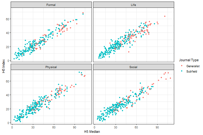
Figure 1. A scatterplot of journal metrics.
Figures — ggplot2 — Notes
geom_point is one of many geoms avilable
- see this https://ggplot2.tidyverse.org/reference for other options, including
geom_barfor bar chartsgeom_boxplotfor box and whiskers plots
Exercises — 24–25
24) Barplot
- see
reproduce_this.pdf: figure 2 on page 7 - apply in
journals.Rmd: figure 2, between paragraphs 21 and 22
25) Scatterplot
- see
reproduce_this.pdf: figure 3 on page 9 - apply in
journals.Rmd: figure 3, between paragraphs 27 and 28
10:00
Tables
Tables — Markdown Syntax
The following syntax, outside code chunks, introduces tables that pandoc can recognise
First Column Second Column ------------ ------------- First cell First cell Second cell Second cell Third cell Third cell| First Column | Second Column |
|---|---|
| First cell | First cell |
| Second cell | Second cell |
| Third cell | Third cell |
Tables — Markdown Syntax
The position of headers, relative to their line underneath, defines column alignments
Left-Aligned Centered ---------------- ----------------First cell First cell Second cell Second cell Third cell Third cell| Left-Aligned | Centered |
|---|---|
| First cell | First cell |
| Second cell | Second cell |
| Third cell | Third cell |
Tables — Markdown Syntax
A line starting with a colon, placed before or after tables, introduces captions
Centered Right-Aligned ---------------- ----------------First cell First cell Second cell Second cell Third cell Third cell : A hand-made table with R Markdown| Centered | Right-Aligned |
|---|---|
| First cell | First cell |
| Second cell | Second cell |
| Third cell | Third cell |
Tables — Markdown Syntax
The caption line itself needs to be surrounded by empty lines
Centered Right-Aligned ---------------- ----------------First cell First cell Second cell Second cell Third cell Third cell : A hand-made table with R Markdown | Centered | Right-Aligned |
|---|---|
| First cell | First cell |
| Second cell | Second cell |
| Third cell | Third cell |
Tables — Markdown Syntax
Tables are numbered automatically
: A hand-made table with R Markdown Centered Right-Aligned ---------------- ----------------First cell First cell Second cell Second cell Third cell Third cell| Centered | Right-Aligned |
|---|---|
| First cell | First cell |
| Second cell | Second cell |
| Third cell | Third cell |
Tables — Markdown Syntax
Grid tables, with the following syntax, can handle complex cells with multiple lines and/or lists
+--------------------+--------------------+| First Column | Second Column | +====================+====================+| - First item | First cell | | - Second item | | | - Third item | |+--------------------+--------------------+|Second cell | Second cell with a | | | long text | +--------------------+--------------------+| Third cell | Third cell | | | | +--------------------+--------------------+: A grid table with multi-line cells| First Column | Second Column |
|---|---|
| - First item - Second item - Third item |
First cell |
| Second cell | Second cell with a long text |
| Third cell | Third cell |
Tables — Markdown Syntax
Grid tables can be aligned as well, with colons at the boundaries of the header separator*
+--------------------+--------------------+| Left-Aligned | Centered | +:===================+:==================:+| - First item | First cell | | - Second item | | | - Third item | |+--------------------+--------------------+|Second cell | Second cell with a | | | long text | +--------------------+--------------------+| Third cell | Third cell | | | | +--------------------+--------------------+: A grid table with multi-line cells| Left-Aligned | Centered |
|---|---|
| - First item - Second item - Third item |
First cell |
| Second cell | Second cell with a long text |
| Third cell | Third cell |
* Use := for left-aligned, :=: for centered, =: for right-aligned columns.
Exercise — 26
26) Markdown Tables
- see
reproduce_this.pdf: table 1 on page 4 - apply in
journals.Rmd: table 1, between paragraphs 11 and 12
05:00
Tables — stargazer — Overview
A capable package for creating at least three kinds of tables
- raw data, in columns and rows
- descriptive/summary statistics
- regression models
Used widely by academics, even tough it has not been updated since 2018
Creates LaTeX code, HTML/CSS code, and ASCII text to be knitted
A lot is written on this package. See, for example,
- the package documentation
- this vignette by its author Marek Hlavac
- this tutorial by Jake Russ
Among its alternatives are the
knitr,kableExtra, andhuxtablepackages
Tables — stargazer — Notes
The
stargazerpackage requires specific settings- in the chunk options
- and, in the
typeargument of thestargazer()function
- These settings depend on the desired output format,* as shown below
| Output | Chunk Option | Type Argument |
|---|---|---|
| LaTex / PDF | results="asis" | latex |
| HTML | results="asis" | html |
| Word | comment="" | text |
* The following slides use the setting for LaTex and PDF outputs.
Tables — stargazer — Notes
stargazertables look slightly different in different output formats- on the following slides, they will have the HTML look
- even if the slides display the setting for LaTex and PDF outputs
In fact, it is currently not quite possible to
knitstargazercode into tables in Word documents- though it can
knitASCII text, looking like a table - some popular workarounds:
knitto HTML as well as Word, copy the tables from HTML to Wordknitto PDF, open the PDF in Word- use a different package to create tables, such as
huxtable
- though it can
Tables — stargazer — Basics
The
stargazer()function- this is probably the only fuction you will ever use from this package
- but it accepts many, many arguments to customise tables
- this is probably the only fuction you will ever use from this package
Tables — stargazer — Basics
The
stargazer()function- this is probably the only fuction you will ever use from this package
- but it accepts many, many arguments to customise tables
- this is probably the only fuction you will ever use from this package
The
dataargument of that function, with two main options- a data frame for data or summary statistics tables
- e.g.,
df, here coming from df <- read_csv(journals.csv)
- e.g.,
- one or more regression models for regression tables
- e.g.,
lm1, here coming from lm1 <- lm(h5_index ~ issues, data = df)
- e.g.,
- a data frame for data or summary statistics tables
Tables — stargazer — Data Tables
Table the first four rows of the dataset
```{r, data_table, echo=FALSE, results="asis"}stargazer(data = head(df, n = 4), type = "latex", summary = FALSE)```Tables — stargazer — Data Tables
Table the first four rows of the dataset
```{r, data_table, echo=FALSE, results="asis"}stargazer(data = head(df, n = 4), type = "latex", summary = FALSE)```Notice the options of the chunk and the arguments of the function
- with echo=FALSE, the code will not be displayed in the output document
Tables — stargazer — Data Tables
Table the first four rows of the dataset
```{r, data_table, echo=FALSE, results="asis"}stargazer(data = head(df, n = 4), type = "latex", summary = FALSE)```Notice the options of the chunk and the arguments of the function
with echo=FALSE, the code will not be displayed in the output document
with results="asis",
knitrwill pass through results without reformatting them- these results are produced in LaTeX, due to type = "latex"
- they should remain LaTeX because our outcome document is PDF, converted from LaTeX
with summary = FALSE, the table will present the data, not its descriptive statistics
Tables — stargazer — Data Tables
Table the first four rows of the dataset
```{r, data_table, echo=FALSE, results="asis"}stargazer(data = head(df, n = 4), type = "latex", summary = FALSE)```% Table created by stargazer v.5.2.2 by Marek Hlavac, Harvard University. E-mail: hlavac at fas.harvard.edu
% Date and time: Fri, Apr 10, 2020 - 12:31:21
| name | origin | branch | h5_index | h5_median | english | subfield | issues | age | |
| 1 | Journal of Bears | Americas | Physical | 73 | 97 | 1 | 1 | 7 | 61 |
| 2 | Journal of Moon | Asia | Social | 72 | 106 | 1 | 0 | 6 | 64 |
| 3 | Journal of Lumber | Americas | Physical | 72 | 100 | 1 | 1 | 8 | 30 |
| 4 | Journal of Houses | Europe | Social | 72 | 102 | 1 | 0 | 8 | 38 |
Tables — stargazer — Data Tables
Set header = FALSE to remove the note preceding tables
```{r, data_table, echo=FALSE, results="asis"}stargazer(data = head(df, n = 4), type = "latex", summary = FALSE, header = FALSE)```| name | origin | branch | h5_index | h5_median | english | subfield | issues | age | |
| 1 | Journal of Bears | Americas | Physical | 73 | 97 | 1 | 1 | 7 | 61 |
| 2 | Journal of Moon | Asia | Social | 72 | 106 | 1 | 0 | 6 | 64 |
| 3 | Journal of Lumber | Americas | Physical | 72 | 100 | 1 | 1 | 8 | 30 |
| 4 | Journal of Houses | Europe | Social | 72 | 102 | 1 | 0 | 8 | 38 |
Tables — stargazer — Data Tables
Define a caption with the title argument
```{r, data_table, echo=FALSE, results="asis"}stargazer(data = head(df, n = 4), type = "latex", summary = FALSE, header = FALSE, title = "First four rows of the dataset")```| name | origin | branch | h5_index | h5_median | english | subfield | issues | age | |
| 1 | Journal of Bears | Americas | Physical | 73 | 97 | 1 | 1 | 7 | 61 |
| 2 | Journal of Moon | Asia | Social | 72 | 106 | 1 | 0 | 6 | 64 |
| 3 | Journal of Lumber | Americas | Physical | 72 | 100 | 1 | 1 | 8 | 30 |
| 4 | Journal of Houses | Europe | Social | 72 | 102 | 1 | 0 | 8 | 38 |
Tables — stargazer — Summary Statistics Tables
Create a table of summary statistics instead, for the complete dataset
```{r, summary_table, echo=FALSE, results="asis"}stargazer(data = df, type = "latex", summary = TRUE, header = FALSE, title = "Descriptive statistics")```| Statistic | N | Mean | St. Dev. | Min | Max |
| h5_index | 1,091 | 26.361 | 13.814 | 1 | 73 |
| h5_median | 1,091 | 39.400 | 21.272 | 3 | 109 |
| issues | 1,091 | 4.676 | 1.786 | 1 | 12 |
| age | 1,091 | 42.902 | 26.370 | 1 | 158 |
Tables — stargazer — Summary Statistics Tables
Keep only a selection of statistics
```{r, summary_table, echo=FALSE, results="asis"}stargazer(data = df, type = "latex", summary = TRUE, header = FALSE, title = "Descriptive statistics", summary.stat = c("n", "mean", "sd", "min", "max"))```| Statistic | N | Mean | St. Dev. | Min | Max |
| h5_index | 1,091 | 26.361 | 13.814 | 1 | 73 |
| h5_median | 1,091 | 39.400 | 21.272 | 3 | 109 |
| issues | 1,091 | 4.676 | 1.786 | 1 | 12 |
| age | 1,091 | 42.902 | 26.370 | 1 | 158 |
Tables — stargazer — Summary Statistics Tables
Omit a selection of statistics for the same effect
```{r, summary_table, echo=FALSE, results="asis"}stargazer(data = df, type = "latex", summary = TRUE, header = FALSE, title = "Descriptive statistics", omit.summary.stat = c("p25", "p75"))```| Statistic | N | Mean | St. Dev. | Min | Max |
| h5_index | 1,091 | 26.361 | 13.814 | 1 | 73 |
| h5_median | 1,091 | 39.400 | 21.272 | 3 | 109 |
| issues | 1,091 | 4.676 | 1.786 | 1 | 12 |
| age | 1,091 | 42.902 | 26.370 | 1 | 158 |
Tables — stargazer — Summary Statistics Tables
Flip the table
```{r, summary_table, echo=FALSE, results="asis"}stargazer(data = df, type = "latex", summary = TRUE, header = FALSE, flip = TRUE, title = "Descriptive statistics", omit.summary.stat = c("p25", "p75"))```| Statistic | h5_index | h5_median | issues | age |
| N | 1,091 | 1,091 | 1,091 | 1,091 |
| Mean | 26.361 | 39.400 | 4.676 | 42.902 |
| St. Dev. | 13.814 | 21.272 | 1.786 | 26.370 |
| Min | 1 | 3 | 1 | 1 |
| Max | 73 | 109 | 12 | 158 |
Exercise — 27
27) Summary Statistics Tables
- see
reproduce_this.pdf: table 2 on page 8 - apply in
journals.Rmd: table 2, between paragraphs 23 and 24
05:00
Tables — stargazer — Regression Tables
Create a table of regression models instead
```{r, regression_table, echo=FALSE, results="asis"}stargazer(data = lm(h5_index ~ issues, data = df), type = "latex", header = FALSE, title = "Regression Results")```| Dependent variable: | |
| h5_index | |
| issues | 1.913*** |
| (0.227) | |
| Constant | 17.415*** |
| (1.137) | |
| Observations | 1,091 |
| R2 | 0.061 |
| Adjusted R2 | 0.060 |
| Residual Std. Error | 13.391 (df = 1089) |
| F Statistic | 70.959*** (df = 1; 1089) |
| Note: | *p<0.1; **p<0.05; ***p<0.01 |
Tables — stargazer — Regression Tables
Models can also be estimated outside the function first
```{r, regression_table, echo=FALSE, results="asis"} lm1 <- lm(h5_index ~ issues, data = df) stargazer(data = lm1, type = "latex", header = FALSE, title = "Regression Results")```| Dependent variable: | |
| h5_index | |
| issues | 1.913*** |
| (0.227) | |
| Constant | 17.415*** |
| (1.137) | |
| Observations | 1,091 |
| R2 | 0.061 |
| Adjusted R2 | 0.060 |
| Residual Std. Error | 13.391 (df = 1089) |
| F Statistic | 70.959*** (df = 1; 1089) |
| Note: | *p<0.1; **p<0.05; ***p<0.01 |
Tables — stargazer — Regression Tables
Keep only a selection of statistics
```{r, regression_table, echo=FALSE, results="asis"}stargazer(data = lm1, type = "latex", header = FALSE, title = "Regression Results", keep.stat = c("n", "rsq"))```| Dependent variable: | |
| h5_index | |
| issues | 1.913*** |
| (0.227) | |
| Constant | 17.415*** |
| (1.137) | |
| Observations | 1,091 |
| R2 | 0.061 |
| Note: | *p<0.1; **p<0.05; ***p<0.01 |
Tables — stargazer — Regression Tables
Display multiple models in the same table
```{r, regression_table, echo=FALSE, results="asis"}stargazer(data = list(lm1, lm2), type = "latex", header = FALSE, title = "Regression Results", keep.stat = c("n", "rsq"))```| Dependent variable: | ||
| h5_index | ||
| (1) | (2) | |
| issues | 1.913*** | 1.424*** |
| (0.227) | (0.212) | |
| english1 | 17.262*** | |
| (1.244) | ||
| Constant | 17.415*** | 4.226*** |
| (1.137) | (1.415) | |
| Observations | 1,091 | 1,091 |
| R2 | 0.061 | 0.202 |
| Note: | *p<0.1; **p<0.05; ***p<0.01 | |
Tables — stargazer — Regression Tables
Change variable labels
```{r, regression_table, echo=FALSE, results="asis"}stargazer(data = list(lm1, lm2), type = "latex", header = FALSE, title = "Regression Results", keep.stat = c("n", "rsq"), dep.var.labels = "H5 Index", covariate.labels = c("Issues", "English"))```| Dependent variable: | ||
| H5 Index | ||
| (1) | (2) | |
| Issues | 1.913*** | 1.424*** |
| (0.227) | (0.212) | |
| English | 17.262*** | |
| (1.244) | ||
| Constant | 17.415*** | 4.226*** |
| (1.137) | (1.415) | |
| Observations | 1,091 | 1,091 |
| R2 | 0.061 | 0.202 |
| Note: | *p<0.1; **p<0.05; ***p<0.01 | |
Tables — stargazer — Regression Tables
Change significance levels
```{r, regression_table, echo=FALSE, results="asis"}stargazer(data = list(lm1, lm2), type = "latex", header = FALSE, title = "Regression Results", keep.stat = c("n", "rsq"), dep.var.labels = "H5 Index", covariate.labels = c("Issues", "English"), star.cutoffs = c(0.05, 0.01, 0.001))```| Dependent variable: | ||
| H5 Index | ||
| (1) | (2) | |
| Issues | 1.913*** | 1.424*** |
| (0.227) | (0.212) | |
| English | 17.262*** | |
| (1.244) | ||
| Constant | 17.415*** | 4.226** |
| (1.137) | (1.415) | |
| Observations | 1,091 | 1,091 |
| R2 | 0.061 | 0.202 |
| Note: | *p<0.05; **p<0.01; ***p<0.001 | |
Exercise — 28
28) Regression Tables
- see
reproduce_this.pdf: table 3 on page 10 - apply in
journals.Rmd: table 3, between paragraphs 30 and 31
07:30
Functionality Gaps
Not everything is possible to achieve with R Markdown syntax, code chunks, and/or code
- e.g., centering text, increasing the space between the lines of text
Functionality Gaps
Not everything is possible to achieve with R Markdown syntax, code chunks, and/or code
- e.g., centering text, increasing the space between the lines of text
Workarounds available through inclusion of other languages and/or syntaxes in .Rmd documents
- e.g., incorporating HTML or LaTeX code into R Markdown
- workarounds might be output specific
- e.g., LaTeX-based workarounds may work only for LaTeX and PDF outputs
There are no exclusive list of gaps or workarounds
- these are specific to the output you want to achieve, problems you encounter
- after writing a few manuscripts with R Markdown, you will have addressed most typical gaps in your workflow
Functionality Gaps — Examples
Problem:
How can we cross-reference figures, tables, and equations in R Markdown?
Solution:
Insert a LaTeX label into the targets (figures, tables, and equations), and then use the \autoref{figure_caption} syntax in text
Functionality Gaps — Examples — Cross-references
For figures, insert a LaTeX label into the fig.caption option, and use the \autoref{latex_label} syntax in text
\autoref{scatter_plot} visualises the relationship between the two journal metrics.```{r ... fig.caption = "A Scatter Plot \\label{scatter_plot}"}ggplot(data = df) + geom_point(...```Figure 1 visualises the relationship between the two journal metrics.
Functionality Gaps — Examples — Cross-references
For Markdown tables, insert a LaTeX label after the table caption, and use the \autoref{latex_label} syntax in text
See \autoref{handmade_table} for further details.: A hand-made table with R Markdown \label{handmade_table}+--------------------+--------------------+| Left-Aligned | Centered | ...See Table 1 for further details.
Functionality Gaps — Examples — Cross-references — Note
Note that there is a difference in the label syntax for figures and R Markdown tables
we use a double backslash \ \ to label figures
e.i., \\label{scatter_plot} because the label goes into a string
the first is an escape operator for the second, LaTeX backslash
we use single backslash \ to label R Markdown tables
e.i., \label{handmade_table} because the label is not in any string
there is no need for the escape operator
Exercises — 29–30
29) Referring to Figures
- see
reproduce_this.pdf: pages 6 and 9 - apply in
journals.Rmd: paragraphs 19, 21, and 27
30) Referring to Markdown Tables
- see
reproduce_this.pdf: page 4 - apply in
journals.Rmd: paragraph 11
05:00
Functionality Gaps — Examples — Cross-references
For stargazer tables, define a label with the label argument, and use the \autoref{latex_label} syntax in text
```{r, regression_table, echo=FALSE, results="asis"}stargazer(data = list(lm1, lm2), type = "latex", ... label = "regression_results")```\autoref{regression_results} provides results from two OLS models.Table 1 provides results from two OLS models.
| Dependent variable: | ||
| H5 Index | ||
| (1) | (2) | |
| Issues | 1.913*** | 1.424*** |
| (0.227) | (0.212) | |
| English | 17.262*** | |
| (1.244) | ||
| Constant | 17.415*** | 4.226** |
| (1.137) | (1.415) | |
| Observations | 1,091 | 1,091 |
| R2 | 0.061 | 0.202 |
| Note: | *p<0.05; **p<0.01; ***p<0.001 | |
Functionality Gaps — Examples — Cross-references — Note
Note that we can cross-reference specific results in tables as well
- there is no gap here — this possible with inline code
In Model 1, the coefficient for _Issues_ is `r round(coef(summary(lm1))["issues", "Estimate"], digits = 2)`.In Model 1, the coefficient for Issues is 1.91.
Functionality Gaps — Examples — Cross-references
For equations, insert a LaTeX label in an equation environment, and use the \autoref{latex_label} syntax in text
\begin{equation}\label{special_relativity}E = mc_{2}\end{equation}According to \autoref{special_relativity}, space and time are linked.According to Equation 1, space and time are linked.
Exercises — 31–33
31) Referring to Tables
- see
reproduce_this.pdf: pages 7 and 9 - apply in
journals.Rmd: paragraph 23 and 29
32) Referring to Results in Regression Tables
- see
reproduce_this.pdf: page 9 - apply in
journals.Rmd: paragraph 29- hint: to extract the standard error from the model, use the column
Std. Error
- hint: to extract the standard error from the model, use the column
33) Referring to Equations
- see
reproduce_this.pdf: page 7 - apply in
journals.Rmd: paragraph 22- hint: transform the existing equation from R Markdown to LaTeX syntax, to be able to insert the label
07:30
Functionality Gaps — Examples
Problem:
R Markdown adds the list of references to the end of documents. This might be undesirable for some manuscripts, for example those with an appendix. Similarly, some journals require tables and figures to be added after references.
Functionality Gaps — Examples
Problem:
R Markdown adds the list of references to the end of documents. This might be undesirable for some manuscripts, for example those with an appendix. Similarly, some journals require tables and figures to be added after references.
Solution:
Define where exactly the list of references should appear with the HMTL code <div id="refs">
# References<div id = "refs"></div># AppendixFunctionality Gaps — Examples
Problem:
R Markdown produces outputs with single-line-spaced text while we might prefer or be required (e.g., by journal submission rules) to double-space our manuscripts.
Solution:
Use the doublespacing command from the LaTeX package setspace (Carlisle, Fairbairns, Harris, and Tobin, 2011)
- because the command comes from a package, we need to add it to YAML with
header-includes - including commands in YAML ensures they are applied through the output*
---...header-includes: - \usepackage{setspace}\doublespacing---* This can be reversed anywhere in text, with the singlespacing command.
Exercise — 34
34) Line Spacing
- introduce 1.5 spacing to the manuscript
- hint: the command is called
onehalfspacing
- hint: the command is called
- except for the Abstract, which should be single spaced
02:00
Functionality Gaps — Examples
Problem:
Pages, tables, figures etc. are numbered continuously across an output. We might prefer or be required (e.g., by journal submission rules) to change this behaviour, for example for appendices.
Solution:
Use the setcounter in combination with the renewcommand command, outside code chunks
\setcounter{page}{1}\renewcommand*{\thepage}{A\arabic{page}}\setcounter{table}{0}\renewcommand*{\thetable}{A\arabic{table}}\setcounter{figure}{0}\renewcommand*{\thefigure}{A\arabic{figure}}Version Control
Research papers have many versions before publication
- typically written over a long period of time, in numerous sittings
- at the end of every sitting, essentially a different version of the same manuscript is created*
* They also often written by multiple authors and/or on different computers, increasing the number of versions created. Here I assume projects are single-authored on a single computer, leaving the topic of collaboration (including, with oneself) to the next section — Part 9.
Version Control
Research papers have many versions before publication
- typically written over a long period of time, in numerous sittings
- at the end of every sitting, essentially a different version of the same manuscript is created
With many versions created over time, there emerge at least two challenges
- keeping track of changes and versions
- reverting to a previous version when necessary
We all version control, in different ways, such as
- edit, rename, and save the files
- use applications or websites such as Dropbox, Google Docs, Overleaf
- use distributed version control systems such as Git and GitHub
Version Control — Manual Attempts
Typically, hand-made attemps to version control lead to cluttered folders
manuscript | |- journals_FINAL_19May.Rmd |- journals_FINAL.Rmd |- journals_26APRIL_newliterature.Rmd ... |- journals.Rproj |- references.bib |- apa_7th.cslVersion Control — Git and GitHub — Definitions
- Git
- a software that keeps track of versions of a set of files
- it is local to you; the records are kept on your computer
Version Control — Git and GitHub — Definitions
- Git
- a software that keeps track of versions of a set of files
- it is local to you; the records are kept on your computer
- GitHub
- a hosting service, or a website, that can keep the records
- it is remote to you, like the Dropbox website
- but unlike Dropbox, GitHub is specifically structured to keep records with Git
- Repository, or repo
- a set of files whose records are kept together, by Git and/or on GitHub
- it is like a folder, which can keep files and other folders containing files
Version Control — Git and GitHub — Definitions
- To commit
- to take a snapshot of, or to version, a repository
- it is like saving a new version of all files and sub-folders in your project folder with a new name
- it is local, the records are kept on your computer unless you push
Version Control — Git and GitHub — Definitions
- To commit
- to take a snapshot of, or to version, a repository
- it is like saving a new version of all files and sub-folders in your project folder with a new name
- it is local, the records are kept on your computer unless you push
- To push
- to move a copy of the records from Git to GitHub, from your computer to online server
- it is like uploading (the new versions of) your files and sub-folders to a website
- it also involves merging, if this not the first push
* For projects that are single-authored on a single computer, merging is typically automatic. It becomes an issue for collaborated projects, which we will cover in the next section — Part 9.
Version Control — Git and GitHub
Version control with Git and GitHub requires
initial setup, done once*
- unless for a new computer or, if ever, a new GitHub account
- a bit technical, but worth the hassle
project setup, repeated for every RStudio project
- shorter, less complicated
* We have started this process already, in Part 1 of the workshop, by downloading and installing Git and signing up for GitHub. Back to the relevant slide.
Version Control — Git — Initial Setup
1) Enable version control with RStudio
- from the RStudio menu, follow:
Tools -> Global Options -> Git/SNV -> Enable version control interface for RStudio projects
RStudio will likely find Git automatically
- In case it cannot do so on its own, help RStudio find it by clicking
Browse... Git is likely to be at
c:/Program Files/Git/bin/git.exeon Windows/usr/local/git/bin/giton Mac
- In case it cannot do so on its own, help RStudio find it by clicking
Version Control — Git — Initial Setup
2) If you are using Windowns, set Git Bash as your shell
- from the RStudio menu, follow:
Tools -> Global Options -> Terminal -> New terminals open with: Git Bash
Version Control — Git — Initial Setup
3) Introduce yourself to Git
- from the RStudio menu, follow:
Tools -> Terminal -> New Terminal
- enter the following lines in the Terminal, with the email address that you have used to sign up for GitHub
git config --global user.name "YOUR-NAME" git config --global user.email "YOUR-EMAIL-ADDRESS"- enter the following line in the Terminal, to observe whether the previous step was sucessful
git config --global --listVersion Control — Git and Github — Project Setup*
1) Initiate local version control with Git
- from the RStudio menu, follow:
Tools -> Version Control -> Project Setup... -> Version Control System -> Git
after confirming your new repository, and restarting the session, observe that
now there is now a Git tab in RStudio
- newly-added and/or edited files, since the last commmit, are listed here
your project now includes a
.gitignorefile- this is where you can list files and/or folders to be excluded from being tracked
* These instructions presume there is an exiting RStudio project to be set up for version control. If not, or to start a new project, follow from this slide first.
Version Control — Git and Github — Project Setup
2) Create a new GitHub repository
- on GitHub, follow:
Repositories -> New -> Repository name (e.g., "rwd_workshop") -> Public -> Create repository
observe the structure of the repository address
- e.i., https://github.com/USER_NAME/REPOSITORY_NAME
- this is the address to view the repository online
- for use in the
Terminal, the address gets the.gitextension
Version Control — Git and Github — Project Setup
3) Push an existing repository
- from the RStudio menu, follow:
Tools -> Terminal -> New Terminal
- enter the following lines in the
Terminal, with your username and repository name
git remote add origin https://github.com/USER_NAME/REPOSITORY_NAME.gitgit add .git commit -m "first commit"git push -u origin masterVersion Control — Git and Github — Project Setup
3) Push an existing repository
- from the RStudio menu, follow:
Tools -> Terminal -> New Terminal
- enter the following lines in the
Terminal, with your username and repository name
git remote add origin https://github.com/USER_NAME/REPOSITORY_NAME.gitgit add .git commit -m "first commit"git push -u origin masterif this is your first time using GitHub with RStudio, you will be prompted to authenticate
- follow the instructions on your screen and in your email
observe that your project files are now online, listed on the GitHub repository
Version Control — Git and Github — Workflow
1) Edit and Save
- work on one or more files under version control
- e.g., delete the first sentence of the abstract in
journals.Rmd, and save it - under the Git tab in RStudio, find the list of files that you edited since the last push
- these will have
M, for modified, asStatus
- e.g., delete the first sentence of the abstract in
2) Commit and Push
- tick
Staged* for one or more files that you would like to commit- enter a
Commit messagethat summarises the edits - click
Committo create a record of the new version locally to your computer - click
Close -> Pushto push the version to GitHub
- enter a
* To stage is to add files to be committed. It allows us to commit files individually or together with other files.
Version Control — Git and Github — Workflow
1) Edit and Save
- work on one or more files under version control
- e.g., delete the first sentence of the abstract in
journals.Rmd, and save it - under the Git tab in RStudio, find the list of files that you edited since the last push
- these will have
M, for modified, asStatus
- e.g., delete the first sentence of the abstract in
2) Commit and Push
- tick
Stagedfor one or more files that you would like to commit- enter a
Commit messagethat summarises the edits - click
Committo create a record of the new version locally to your computer - click
Close -> Pushto push the version to GitHub
- enter a
- observe the changes in the Git tab in RStudio and on the GitHub repository
Version Control — Git and Github — .gitignore
.gitignorespecifies which file(s) and/or folder(s) should be excluded from version control- a set of project-specific files are ignored by default
- see your
.gitignorefile
- see your
- a set of project-specific files are ignored by default
Version Control — Git and Github — .gitignore
.gitignorespecifies which file(s) and/or folder(s) should be excluded from version control- a set of project-specific files are ignored by default
- see your
.gitignorefile
- see your
- a set of project-specific files are ignored by default
.gitignorelists one item per line- each line has a pattern, which determines whether one or more files or folders are to be ignored
See the documentation at https://git-scm.com/docs/gitignore
- for pattern formats and further details
Version Control — Git and Github — .gitignore
There are good reasons to ignore some others, including files
- that contain information that we do not want others to see
- e.g., personal API keys
- e.g., personal API keys
- that we do not have the right to share with others
- e.g., secondary data with user agreements otherwise
- e.g., secondary data with user agreements otherwise
- that we (re-)create automatically as outputs
- e.g.,
journals.pdf, as opposed to journals.Rmd
- e.g.,
Version Control — Git and Github — .gitignore
- Observe that, by default,
.gitignorehas a list of project-specific files- you can delete, or comment out, any or all to start including them in version control
.Rproj.user.Rhistory.RData.RuserdataVersion Control — Git and Github — .gitignore
Observe that, by default,
.gitignorehas a list of project-specific filesIn addition, you can ignore, for example,
- a specific folder, relative to the root directory
.Rproj.user.Rhistory.RData.Ruserdata/manuscript/Version Control — Git and Github — .gitignore
Observe that, by default,
.gitignorehas a list of project-specific filesIn addition, you can ignore, for example,
a specific folder, relative to the root directory
a specific file in a specific folder, relative to the root directory
.Rproj.user.Rhistory.RData.Ruserdata/manuscript//manuscript/journals.pdfVersion Control — Git and Github — .gitignore
Observe that, by default,
.gitignorehas a list of project-specific filesIn addition, you can ignore, for example,
a specific folder, relative to the root directory
a specific file in a specific folder, relative to the root directory
a specific file in any folder
.Rproj.user.Rhistory.RData.Ruserdata/manuscript//manuscript/journals.pdfjournals.pdfVersion Control — Git and Github — .gitignore
Observe that, by default,
.gitignorehas a list of project-specific filesIn addition, you can ignore, for example,
a specific folder, relative to the root directory
a specific file in a specific folder, relative to the root directory
a specific file in any folder
all files with a specific extension, anywhere in the project
.Rproj.user.Rhistory.RData.Ruserdata/manuscript//manuscript/journals.pdfjournals.pdf *.pdfVersion Control — Git and Github — .gitignore — Notes
There are many other pattern formats
- see the documentation at https://git-scm.com/docs/gitignore
Version Control — Git and Github — .gitignore — Notes
There are many other pattern formats
- see the documentation at https://git-scm.com/docs/gitignore
Starting to ignore a file or folder that is already being tracked requires clearing the cache
- after changing and saving
.gitignore, enter the following line in theTerminal - with your speficic
/path/to/file
- after changing and saving
git rm --cached /path/to/fileVersion Control — Git and Github — .gitignore — Notes
There are many other pattern formats
- see the documentation at https://git-scm.com/docs/gitignore
Starting to ignore a file or folder that is already being tracked requires clearing the cache
- after changing and saving
.gitignore, enter the following line in theTerminal - with your speficic
/path/to/file
- after changing and saving
git rm --cached /path/to/fileThe following command clears all cache
- might be useful after changes to
.gitignorethat involves several files or folders - but should be used with care, on an otherwise up-to-date repository
- might be useful after changes to
git rm -r --cached .Exercises — 35–36
35) Reproducibility and Version Control
- imagine that, after producing all these tables and figures, and writing up your results, you have decided to exclude journals from Oceania from analysis
- hint: use the
filterfunction in the data chunk - create a new version of the manuscript
- commit and push to GitHub
- hint: use the
36) Gitignore
- stop tracking
journals.pdf- change
.gitignore - remove
journals.pdffrom cache - commit and push to GitHub
- change
05:00
Collaboration
Many research papers are written by multiple authors and/or on multiple computers
- yourself on a different computer (e.g., laptop at home, desktop at office), poses similar challenges as collaboration
Collaboration
Many research papers are written by multiple authors and/or on multiple computers
- yourself on a different computer (e.g., laptop at home, desktop at office), poses similar challenges as collaboration
With multiple authors and/or computers, there emerges at least two additional challenges beyond version control
- communicating the versions to other authors and/or computers
- working on the same project with co-authors at the same time
We all manage collaboration, in different ways, such as
- edit, rename, save, e-mail
- use applications or websites such as Dropbox, Google Docs, Overleaf
- use distributed version control systems such as Git and GitHub
Collaboration — Git and GitHub — Definitions
To pull
- to move the (presumably) up-to-date records from GitHub to your computer
- it is like downloading a zipped folder of files
Collaboration — Git and GitHub — Definitions
To pull
- to move the (presumably) up-to-date records from GitHub to your computer
- it is like downloading a zipped folder of files
To merge
- to integrate different versions into a single version
- e.g., the old version on your laptop, with (the changes in) the new version from GitHub
- except the first push or pull, pushing and pulling necessiate merging
- to integrate different versions into a single version
Merge conflict
- emerges when versions to be merged include edits on the same line of the same file
- edits on different lines are not a problem as changes are tracked line by line
- edits on different lines are not a problem as changes are tracked line by line
- less likely to occur in one-author-multiple-computer setting
- more likely while collaborating with others
- more likely while collaborating with others
- requires human intervention, to decide which edit to keep and which one to discharge
- emerges when versions to be merged include edits on the same line of the same file
Collaboration — Git and GitHub — Definitions
Branch
- a line of development in a repository; a copy of the repository, with all its versions, at a given time
- by default, repositories have one branch, called master
Pull request
- a proposal to pull and merge
- e.g., a proposal from one co-author to another, -e.g., tp merge a branch into master
- it allows a review of changes on GitHub before merge, to deal with potential merge conflicts
- a proposal to pull and merge
Collaboration — Git and GitHub — Project Setup
- The setup depends on the users' role, on whether they are
- the owner who creates the GitHub repository, or
- the collaborator who is then added to that repository
Collaboration — Git and GitHub — Project Setup
- The setup depends on the users' role, on whether they are
- the owner who creates the GitHub repository, or
- the collaborator who is then added to that repository
- Once the project is setup
- it continues to be associated with the owner's GitHub profile
- at the same time, it is listed under the collaborator's profile as well
- both the owner and the collaborator have the same rights, unless otherwise restricted
Collaboration — Git and GitHub — Project Setup — Owner
1) The setup for the owner is largely the same as in any single-author, single-computer scenario
- following the instructions on this slide forward
- to introduce version control to a local project with Git,
- to create a remote repository for that project on GitHub, and
- to associate the local project with the remote repository
2) As an additional step, the owner needs to invite their collaborator(s) to the project
- following, from the relevant GitHub repository,
Settings -> Manage access -> Invite a collaborator
Collaboration — Git and GitHub — Project Setup — Collaborator
1) Notice that the remote part of the setup is done by the owner for the collaborator
- subject to acceptance of the invitation
- invitations are available directly at https://github.com/notifications, but also sent via email
- with an option to "Accept invitation"
- on acceptance, projects appear among the repositories of the collaborator
2) The local part of the setup still needs to be done
- by creating a new RStudio project with version control
- following, from the Rstudio menu,*
File -> New Project -> Version Control -> Git
- the
Repository URL, required for the above process, is the version without the.gitextension- in the form of https://github.com/OWNER_USER_NAME/REPOSITORY_NAME
Exercises — 37–39
37) Owner Setup
- create a new version-controlled RStudio project, with Git and GitHub
- add the default R Markdown template to your project
- hint: click
File -> New File -> R Markdown -> OKto create the template - another hint: name the project and the template in a way that they are easily distinguishable from your partner's project and template
- hint: click
38) Invitation to Collaborate
- invite the partner in your current group as a collaborator to your new project
- hint: you will need their username, full name, or email address to do so
39) Collaborator Setup
- accepting the invitation from your partner, do the necessary arrangements so that you can collaborate on your partner's project
10:00
Colloboration — Git and Github — Workflow
1) Pull
- on the Git tab in RStudio, click
Pullto move the up-to-date records from GitHub to your computer- if your collaborator has not pushed anything since your last pull, you will be noticed that
Already up-to-date. - collaborative projects require pulling as well as pushing because your collaborator(s) might have pushed their commits to GitHub
- pulling frequently minimises the risk of merge conflicts
- if your collaborator has not pushed anything since your last pull, you will be noticed that
2) Edit and save; commit and push
- the same procedure as in any single-author, single-computer scenario
- as described on this slide forward
- pushing frequently minimises the risk of merge conflicts
Exercise — 40
40) Non-simultaneous Collaboration
take in turns with your partner to work on the same document (of the same project)
owner: edit the first header in the document (i.e., "R Markdown"), save, commit, and push
owner and collaborator: observe the changes, if any, on your own
.Rmdfile, and/or on your GitHub repository- click on the relevant commit message on GitHub and observe the commit
collaborator: pull, revert the header back to original, save, commit, and push
05:00
Exercise — 40 — Notes
Notice that you have not encountered any errors and/or merge conflicts
because everyone edited and merged with an up-to-date document
this is the default scenario in single-author, multiple computer scenario
Exercise — 41
41) Simultaneous Collaboration — Different Lines
- work on the same document at the same time
- owner: edit the first header in the document (i.e., "R Markdown"), save, commit, and push
- collaborator: edit the second header in the document (i.e., "Including Plots"), save, commit, and push
- observe the error message that the last pusher will receive, follow the instructions on RStudio to solve the problem
10:00
Exercise — 41 — Notes
Notice that you have encountered an error
pulling before pushing solves the problem because the edits are not on the same line
- hence, this is not a merge conflict
the merge takes place automatically, on the local repository of the last pusher
Exercise — 42
42) Simultaneous Collaboration — Same Line
work on the same document at the same time
owner: edit the first header in the document again, save, commit, and push
collaborator: edit the first header in the document as well, save, commit, and push
observe the error message that the last pusher will receive
- follow the instructions on RStudio to solve the problem
- google if necessary
10:00
Exercise — 42 — Notes
Notice that you have encountered not only an error but also a merge conflict
pulling before pushing alone does not solve the problem because the edits are on the same line
- the conflict cannot be solved automatically — it needs human intervention
nevertheless, by pulling first, you can view the conflict directly on the file
- marked between less than < and greater than > signs, divided by the equal signs
- solution is to accept the remote version, by deleting your edit and or moving that edit to a different line
the merge takes place on the local repository of the last pusher
Colloboration — Git and Github — Workflow — Alternative
- The workflow above is rather simple, but has some disadvantages, including
- not easy, albeit still possible, to see the edits of the collaborators
- not clear who is in charge of the overall progress
- not possible to discuss edits
- not possible to compromise on conflicting edits
- An alternative workflow exits
- work on different branches of the same project
- version control to your own branch
- create pull requests with comments
- merge the branch into master
Colloboration — Git and Github — Workflow — Alternative
1) Branch
- click
New Branchon the Git tab- name it, and leave everything else as default
- notice that you are now working on a new branch
2) Edit and save; commit and push
- the same procedure as in any single-author, single-computer scenario
- as described on this slide forward
- notice, on GitHub, that your commit is in the new branch, while master remains unchanged
3) Pull request
On GitHub, click
Pull requests -> New pull requestchoose what is to be pulled, and write a note to your collaborator who can accept or reject the merge
- if there are merge conflicts, the collaborator solves them on GitHub before merging
Exercises — 43–44
43) Pull request
- create a pull request for your collaboration project
- create a branch for yourself
- edit any line, save, commit, and push
- request your branch to be merged
44) Merging
- view the pull request of your collaborator
- take the necessary steps to merge it to master
10:00
Colloboration — Git and Github — Workflow — Notes
It is possible to edit
.Rmddocuments directly on GitHub- click on any editable file, and
Edit this file - commit changes, either as a direct commit or a pull request
- click on any editable file, and
Colloboration — Git and Github — Workflow — Notes
It is possible to edit
.Rmddocuments directly on GitHub- click on any editable file, and
Edit this file - commit changes, either as a direct commit or a pull request
- click on any editable file, and
A GitHub account is enough for collaboration with co-authors who do not work with Git, R, or RStudio
- not possible to knit to see the outcome
- would suit co-authors whose contributions are plain text
Exercises — 45
45) GitHub edit
- create two edits on the
.Rmddocument in your collaboration project - commit one of the edits as a direct commit
- commit the other as a pull request
05:00
Real Project
Consider converting a real project to R Markdown
- now, in the remainder of the workshop
Choose an existing project, preferably
- single-authored
- at an early stage
- but one that you are, will be, working on
Ask me for help
- with no more slides to go through, I will now focus on helping you start your first project in R Markdown
References
Allaire, J., Y. Xie, J. McPherson, et al. (2022). rmarkdown: Dynamic Documents for R. R package version 2.14. <https://CRAN.R-project.org/package=rmarkdown.
Blair, G., J. Cooper, A. Coppock, et al. (2022). fabricatr: Imagine Your Data Before You Collect It. R package version 0.16.0. <https://CRAN.R-project.org/package=fabricatr.
Carlisle, D., R. Fairbairns, E. Harris, et al. (2011). setspace – Set space between lines. LaTeX package, version 6.7a. <https://ctan.org/pkg/setspace.
Dowle, M. and A. Srinivasan (2021). data.table: Extension of
data.frame. R package version 1.14.2.
<https://CRAN.R-project.org/package=data.table.
Gagolewski, M., B. Tartanus, o. Unicode, et al. (2021). stringi: Character String Processing Facilities. R package version 1.7.6. <https://CRAN.R-project.org/package=stringi.
Hlavac, M. (2022). stargazer: Well-Formatted Regression and Summary Statistics Tables. R package version 5.2.3. <https://CRAN.R-project.org/package=stargazer.
Hugh-Jones, D. (2021). huxtable: Easily Create and Style Tables for LaTeX, HTML and Other Formats. R package version 5.4.0. <https://hughjonesd.github.io/huxtable/.
References
R Core Team (2022). R: A Language and Environment for Statistical Computing. R Foundation for Statistical Computing. Vienna, Austria. <https://www.R-project.org/.
Sievert, C., C. Parmer, T. Hocking, et al. (2021). plotly: Create Interactive Web Graphics via plotly.js. R package version 4.10.0. <https://CRAN.R-project.org/package=plotly.
Wickham, H., R. François, L. Henry, et al. (2022). dplyr: A Grammar of Data Manipulation. R package version 1.0.9. <https://CRAN.R-project.org/package=dplyr.
Wickham, H. and G. Grolemund (2021). R for data science. O'Reilly.
Xie, Y. (2022a). bookdown: Authoring Books and Technical Documents with R Markdown. R package version 0.26. <https://CRAN.R-project.org/package=bookdown.
Xie, Y. (2022b). knitr: A General-Purpose Package for Dynamic Report Generation in R. R package version 1.39. <https://yihui.org/knitr/.
Xie, Y. (2022c). tinytex: Helper Functions to Install and Maintain TeX Live, and Compile LaTeX Documents. R package version 0.39. <https://github.com/rstudio/tinytex.
References
Xie, Y., J. Allaire, and G. Grolemund (2018). R Markdown: The Definitive Guide. ISBN 9781138359338. Boca Raton, Florida: Chapman and Hall/CRC. <https://bookdown.org/yihui/rmarkdown.
Xie, Y., C. Dervieux, and A. Presmanes Hill (2022). blogdown: Create Blogs and Websites with R Markdown. R package version 1.10. <https://CRAN.R-project.org/package=blogdown.
Zhu, H. (2021). kableExtra: Construct Complex Table with kable and Pipe Syntax. R package version 1.3.4. <https://CRAN.R-project.org/package=kableExtra.